Download
1 / 9
90 likes | 235 Views
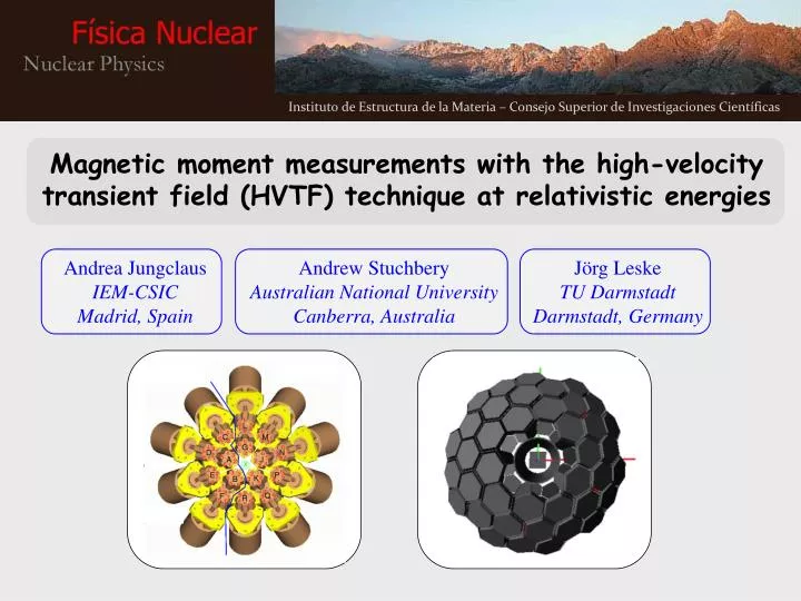
Instituto de Estructura de la Materia – Consejo Superior de Investigaciones Científicas. Magnetic moment measurements with the high-velocity transient field (HVTF) technique at relativistic energies.

E N D
Instituto de Estructura de la Materia – Consejo Superior de Investigaciones Científicas Magnetic moment measurements with the high-velocity transient field (HVTF) technique at relativistic energies Andrea Jungclaus IEM-CSIC Madrid, Spain Andrew Stuchbery Australian National University Canberra, Australia Jörg Leske TU Darmstadt Darmstadt, Germany
Why to measure magnetic moments of short-lived excited states in exotic nuclei ? One example … B(E2) anomaly in 136Te Exp. and theoretical g(2+) in Te the isotopes 136Te Te 136Te N. Benczer-Koller et al., PLB 664(2008)241 D.C. Radford et al., Phys. Rev. Lett. 88 (2002) 222501 g-factor is very sensitive to relative proton (neutron) composition of nuclear wavefunction !
How to measure magnetic moments ? Larmor frequency L = g · N/ħ · B MTesla ! Time integral measurement of the precession angle /g = N/ħ·B·teff kT fields required for short teff (<t) ! kTesla ! Fermi contact field [Tesla] Magnetic fields of this strength in general available at the nucleus ONLY due to its own electrons ! Fermi contact field at the nucleus: B1s = 16.7 Z3 R(Z) [T] for 1s electrons H O F Ne Mg Si Xe R(Z) 1+(Z/84)2.5 relativistic correction factor randomly oriented electron spins: attenuation of g-ray angular distribution “nuclear deorientation” oriented electron spins (polarization): precession of g-ray angular distribution “transient fields”
Three different techniques to measure g-factors of short-lived states using radioactive beams nuclear deorientation low-velocity transient field 132Te @ Oak Ridge 3.0 MeV/u N.J. Stone, A.E. Stuchbery et al., Phys. Rev. Lett. 94 (2005) 192501 high-velocity transient field 132Te @ Oak Ridge 3.0 MeV/u N. Benczer-Koller et al., PLB 664(2008)241 38,40S @ MSU 40 MeV/u A.D. Davies et al., PRL 96 (2006) 112503 A.E. Stuchbery et al., PRC 74 (2006) 054307 138Xe @ REX-ISOLDE 2.8 MeV/u 2006/2009 SP: A. Jungclaus, J. Leske 72Zn @ GANIL 60 MeV/u April 2008 SP: G. Georgiev, A. Jungclaus 42,44,46Ar @ MSU & N=40 Fe @ MSU October 2008 SP: A.E. Stuchbery Nothing yet at relativistic energies ! Only very few experiments so far advantages and disadvantages of the different techniques still need to be explored !
Transient field strength in Fe host Transient fields: From the low- to the high-velocity regime ξ1s: degree of polarization of 1s electrons F11s: ion fraction with unpaired 1s electrons B1s: Fermi contact field of 1s electrons Btf (v, Z) = ξ1s(v, Z) · F11s(v, Z) · B1s(Z) v/c20-50% Z∙v0: 1s electron velocity intermediate-energy & relativistic Coulex maximum around v=Z∙v0 strength scales with Z3 (Z2 in Gd) v/c3-7% Problem: Transient field strength studied only up to Sulfur (in Canberra). What happens for higher Z ? low-energy Coulex A.E. Stuchbery et al., Phys. Rev. C74 (2006) 054307 Phys. Lett. B611 (2005) 81 30 shifts of parasitic 136Xe beam approved by GSI PAC in 2009 calibration of TF strength in the 132Sn region !
How to measure the precession of a g-ray angular correlation with the PRESPEC setup ? 134Te 136Xe primary beam @ 500 MeV/u 2.5 g/cm2 Be target 134Xe LYCCA-0 Wlab(Q) 4.1 ps 62 MeV/u 1.5º 134Xe 400 mg/cm2 Gd 2.1º 100 MeV/u 0.1º-1.7º 83.5 MeV/u 2.3 ps t(2+)=3.0(2) ps figure of merit Including decay: teff = 1.4 ps, v/Zv0 = 1.07-0.93 Snuc(Q), S2N Df/g = 129 mrad, Bave = 1.9 kTesla N=7500 photopeak counts per field per day in Clusters A, D and E Only angular range 40º and 120º useful for precession measurement ! Full simulation performed using the code GKINT by A. Stuchbery angle Q (deg)
B Geometry of the PRESPEC Ge array PRESPEC P 10o 40o ! E 134Te A D N J The RISING array isverywellsuited forsuch a precessionmeasurement ! All Ge crystals in the range 40º and three pairs of Cluster detectors close to the horizontal plane!
From the RISING@GSI to the AGATA@GSI setup In case of a successful calibration experiment with the RISING setup we would like to tackle a first physics case in the 132Sn region with the AGATA@GSI setup ! standard configuration C. Domingo It is still under study whether a larger than the standard distance would lead to a higher sensitivity to the precession.
Summary & Conclusions Magnetic moment information is important (sometime E(2+) and B(E2) is not sufficient) ! Transient fields (TF) largest around 1s electron velocity Relativistic heavy ions “in principle” well suited for g(2+) measurements ! TF strength only known up to Z=16 (30) We need at least one calibration point to tackle the 132Sn region. Approved parasitic beamtime at GSI ! GSI only ! Once the TF strength is known real physics cases in the 132Sn region can be studied with the AGATA@GSI setup !