Download
1 / 65
680 likes | 835 Views
Designs for Muon Tomography Station Prototypes Using GEM Detectors. Leonard V. Grasso III Advisor: Dr. Marcus Hohlmann April 13, 2012. The Discovery of the Muon. The origins of the history of the muon can be traced back to the era from 1930 to 1950.

E N D
Designs for Muon Tomography Station Prototypes Using GEM Detectors Leonard V. Grasso III Advisor: Dr. Marcus Hohlmann April 13, 2012
The Discovery of the Muon • The origins of the history of the muon can be traced back to the era from 1930 to 1950. • Hideki Yukawa proposed the first significant theory of the strong nuclear force in 1934. He predicted that the strong field should be quantized, and that its mediator should be a particle about 300 times as massive as an electron. • In 1937, the discovery of a new particle by Street and Stevenson was not only thought to be what Yukawa was looking for, but also helped to vindicate quantum electrodynamics.
However, as time went on, disturbing discrepancies arose between Yukawa’s predictions and observed experimental results. The observed particles had the wrong lifetime, were lighter than predicted, and in 1946 were shown to interact weakly with atomic nuclei. In 1947, Powell showed that two particles were being detected that were derived from cosmic rays: the muon (observed by Street and Stevenson), and the pion. Neither, however, was what Yukawa was looking for. The Discovery of the Muon
The Discovery of the Muon • Of all the products of high energy collisions in our atmosphere, it is primarily muons that can be observed at the surface of the Earth. • The muon’s lifetime on average is about 2.2×10⁻⁶ s. Assuming that muons are produced at about 8,000 m above sea level and travel at about 0.998c, special relativity is required to explain them reaching Earth’s surface. • According to classical kinematics, they should not reach the surface: • According to relativistic kinematics, we observe muons to have an increased lifetime on average. The increased lifetime allows muons to penetrate well below the surface of the Earth.
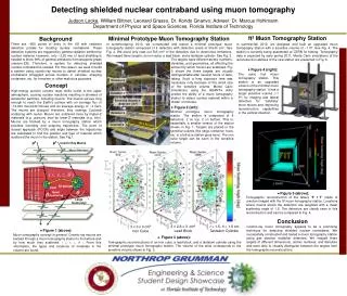
Imaging Techniques Using Muons Since the discovery of the muon, scientists have sought ways to exploit the constant, free supply that goes through us all the time. I will mention two imaging techniques that have been developed using them. • The first is called shadow radiography and was pioneered by Luis Alvarez in the 1960’s to search for hidden chambers in the ancient Egyptian pyramid of Chephren. • The second is called muon tomography (MT) and was developed by Christopher Morris at Los Alamos National Lab in 2001. In 2003, LANL started to explore the use of MT to detect smuggled nuclear material (SNM) at our nation’s ports and borders.
Imaging Techniques Using Muons • Shadow radiography uses detectors to compare the number of incident muons in certain areas against others. Alvarez’s detectors consisted of a series of spark chambers, trigger counters, and 36 tons of iron. • The figure to the left shows relatively uniform muon counts. The figure to the right shows an area with higher than usual counts, which would be indicative of more muons being able to pass through a less dense or possibly hollow volume there.
Imaging Techniques Using Muons • Although muons have high penetrating properties, they do interact with matter to some degree via coulomb scattering. Muons are scattered more by atoms with large atomic numbers than they are by atoms with small atomic numbers. • MT uses detectors to track incoming and outgoing velocity vectors of muons and uses an algorithm that can calculate the position that a deflection occurred, along with a scattering angle, thereby revealing the location and density of material. • To date, drift tubes, developed by Georges Charpak, and gas electron multiplier (GEM) detectors, developed by Fabio Sauli, have been used in MT. Our group is the first to use GEM detectors to that end.
Gas Electron Multiplier Detectors • GEM detectors are micro-pattern gas detectors used for the detection of charged particles, such as muons. • Muons passing through a detector ionize the gas filling it in the drift region. The freed electrons are then accelerated through a series of GEM foils that have a potential difference across them, further ionizing the gas and producing an avalanche of electrons. • The avalanche of electrons induces a current in the detector’s readout, revealing the position that a muon crossed the detector.
Gas Electron Multiplier Detectors • Honeycomb frame • Drift Cathode • Foils (referred to as GEM foils) • Readout • Gas mixture filling the volume of each detector Each GEM detector has five basic components: The figure on the left shows a magnified view of the micro-pattern holes etched into each GEM foil. On the right, one sees that the conical shape of these holes helps to concentrate the electric field lines filling them.
Gas Electron Multiplier Detectors • The honeycomb frame serves to provide strong structural integrity while minimizing the amount of material required to do so. • The drift cathode has a negative potential applied across it to attract positive ions created in the ionization process. • Typically two or three GEM foils are used in each detector. A potential difference is applied across them, and freed electrons are accelerated through them further ionizing the gas in the detector (electron multiplication). • A readout is placed at the bottom of each detector and measures the amplified signal produced to determine the position at which an interaction occurred. • Our detectors are filled with an argon / carbon dioxide mixture (70:30). This mixture is cost efficient, relatively easy to ionize, facilitates and recovers quickly from electron avalanching, and is non-corrosive.
Muon Tomography Station Prototype I • One of the long term goals of our research group is to design and commission large scale MT stations using GEM detectors that can be used to image cargo containers at our nation’s ports and stop SNM more efficiently and less expensively than is currently done. • By 2008 our group had run exhaustive simulations which suggested that this goal is feasible. • In 2009 we were ready to collect real data from physical detectors, and I was tasked to design and build our group’s MTS prototype I. • A framework needed to be designed to mount detector stacks around an imaging volume. A minimum of two detectors are required in a detector stack because each detector reads out a point in space where a muon crossed it. • In 2009 we only had enough detectors to employ stacks on the top and bottom of the imaging volume. Therefore, I designed our MTS prototype I to accommodate top and bottom detector stacks only.
Muon Tomography Station Prototype I • The primary structural components of our MTS prototype I are a base plate used to support four ¼-20 threaded stainless steel rods and a target plate. 6061-T6 aluminum alloy was used to machine them. • SolidWorks, a 3D mechanical CAD program, was used to model the prototype, as well as detector assemblies, to test for feasibility and to make final improvements before production. • Left figure: Top view of prototype I using SolidWorks with simulated elements of the top detector assembly in the top stack. Right figure: 3D view of MTS prototype I.
Muon Tomography Station Prototype I • Left figure: Actual base plate used in our MTS prototype I. Its dimensions are 20 in x 22 in x ¾ in. The cylinders have an outer diameter of ¾ in, an inner diameter of ¼ in, and a height of 3.0 in. Steel support rods screw into them 1.5 in deep. • Right figure: The target plate used in our MTS prototype I. Its dimensions are 20 in x 22 in x 3/8 in. The engraved square denotes the boundary of the imaging volume.
Muon Tomography Station Prototype I • Left figure: MTS prototype I with mock readouts and imaging material. The readout at the top of the top stack was an actual readout that had been damaged. • Right figure: Fully commissioned MTS prototype I collecting data at CERN. Note that two GEM detectors are being used in each detector stack, and a small block of lead is being imaged. The damaged readout is able to serve as the target plate here.
Muon Tomography Station Prototype II • During 2010, more detectors were being commissioned and becoming available to use. That year I designed and built our prototype II station. • A key requirement of the new design was that detector stacks on four sides of the imaging volume needed to be accommodated. Simulations showed that adding side detector stacks to our imaging station should dramatically improve its coverage. • Above: Coverage is the imaging station’s ability to track muons passing through all subvolumes of the imaging volume. For a muon’s track to count (or be measured), it must pass through two detector stacks.
Muon Tomography Station Prototype II • An imaging station with detector stacks on four sides should be a big improvement over the prototype I station, but the design of such a station would have to be very different. • Detectors would have to be mounted to support plates via fixation holes in their readouts, the support plates would have to be big enough to allow for the space needed by electronics and other components, and the support plates would have to be mounted in the prototype II station. • Left figure: PVC plate used to support GEM detectors and their readouts. The support plates have dimensions of ¼ in x 19 in x 26 in. Right figure: Simulated view of a detector assembly mounted to its support plate using SolidWorks.
Muon Tomography Station Prototype II • Support plates had to overlap so that active areas of the GEM detectors defined the imaging volume. With that constraint in mind, I tried to imagine an imaging station, or framework, built around that geometry. • My prototype II design consists of extruded angles and T-bars made of 6061-T6 aluminum alloy welded together to make four quadrants. • The four quadrants of the framework are bound together by smaller extruded angles screwed into it used to support top and bottom detector stacks, as well as support brackets connected to them using nuts and bolts for maximum stability.
Muon Tomography Station Prototype II • Left figure: An extruded angle used to construct quadrant one of the prototype II imaging station. The L shape is 1.5 in x 0.75 in and is 0.125 in thick, and the angle itself is 15.5 in long. The holes are 0.113 inches in diameter, are 0.25 in apart, and are used to fixate the PVC detector support plates. • Right figure: A T-bar used to construct quadrant one of the prototype II imaging station. The T shape is 1.5 in x 1.5 in and is 0.188 in thick, and the bar itself is 15.5 inches long. The holes are 0.113 inches in diameter, are 0.25 in apart, and are used to fixate the PVC detector support plates.
Muon Tomography Station Prototype II Quadrant one of our MTS prototype II. Elements one and two are extruded angles, and elements three and four are T-bars. Element five is simply an aluminum base plate used for support, and element six is an extruded angle with no holes also used to support the framework. Note that the vertical extruded angle and T-bar have twin sets of holes. One set is used to screw into extruded angles which support detector assemblies in top and bottom detector stacks, and the other set is used to fixate PVC plates. The sets of twin holes are separated by half an inch. All elements shown are welded together to form a solid and stable assembly.
Muon Tomography Station Prototype II • Quadrants one and two of our MTS prototype II imaging station. Quadrant two is composed of the same fundamental elements as quadrant one, and they are arranged to accommodate the geometry shown previously. In a similar fashion, quadrants three and four are constructed.
Muon Tomography Station Prototype II • Simulated MTS prototype II imaging station complete with all four quadrants, four detector stacks, and target plate with material to be imaged. The completed station is approximately 47 inches long by 29 inches wide by 42 inches high.
Muon Tomography Station Prototype II • Assembled MTS prototype II in Florida Tech’s machine shop shortly after its construction was completed in June 2010. The station is loaded with PVC support plates that will be used to secure GEM detectors and scintillators, along with their supporting electronics.
Muon Tomography Station Prototype II • Assembled MTS prototype II in Florida Tech’s High Energy Physics Lab A. Along with PVC support plates, the station is also loaded with target plates secured by C-clamps and mock material to be imaged.
Muon Tomography Station Prototype II • Partially loaded MTS prototype II at CERN. Top and bottom detector stacks are fully loaded, but side detectors have not been mounted yet. A target plate with material to be imaged is also missing.
Muon Tomography Station Prototype II • Fully loaded MTS prototype II in Florida Tech’s High Energy Physics Lab A. Detector stacks are mounted on all four sides, and one can see the material being imaged in the center of the imaging volume.
Photon Attenuation Calculation • The primary materials used for nuclear fission weapons are U-235 and Pu-239. I chose to simulate how effective our station would be at detecting U-235 encased in lead shielding. • The most probable gamma emitted by U-235 has an energy of 186 keV. The figure above gives the photon mass attenuation length for various elements, including lead, as a function of photon energy.
Photon Attenuation Calculation Given the density of lead is ρ = 11.34 g/cm3, the photon mass attenuation length for a gamma of energy 186 keV traveling through lead is λ = 0.8 g/cm2, Io is the initial intensity of the photon, and I(x) is the intensity of the photon remaining after traveling a distance x in cm through the material, the following formula can be used to calculate the thickness of lead needed to absorb 99.9% of all gammas with energy 186 keV: Therefore, a lead box of thickness 5 mm would be capable of shielding over 99.9% of the most probable gammas emitted from U-235, and I will simulate U-235 in such a shield in the following scenarios.
All simulations run are subject to the following parameters: Analysis of Simulated Scenarios Full cubic foot station 3 m x 3 m CRY (Cosmic RaY) plane MTS (Muon Tomography Station) volume is air In the images of my analysis that follow, all data in the perpendicular coordinate is collapsed into the plane shown. Degrees shown in images provide a fourth dimension of analysis and refer to the scattering angle of muons passing through material. In Root plots analyzing the simulated POCA (Point Of Closest Approach), a cut of 3 degrees and a maximum value of 8 degrees is used for each scenario. All scattering angles below the cut angle are not shown, and all scattering angles above the maximum angle are shown as the maximum angle.
Analysis of Simulated Scenarios = number of events The cosmic muon flux at sea level is 1x10⁴ events per square meter per minute. Since the Geant4 code used for my simulations is run in event space, this flux can be used in the following table to determine how many events correspond to an actual amount of real exposure time. For my simulations, I chose to analyze exposure times of 1 minute, 4 minutes, 10 minutes, 60 minutes, and 600 minutes. The number of events that correspond to the above exposure times are calculated on the following slide. In this presentation, I will comment on the images produced with 600 minutes of exposure time. Note that in the configuration file for my simulations, a nine square meter CRY plane was specified. It should also be noted that Root was used to analyze the output of my Geant4 simulations, and the required number of events for each exposure time could be specified in the Root configuration file.
Analysis of Simulated Scenarios • Above is shown the detector geometry used in my simulations, which matches the detector geometry in our MTS prototype II.
Geometry of shielded scenario xy: z = -110 mm, z = 0 mm, and z = 110 mm viewed in the xy plane. The positive z axis is pointing out of the screen. y-axis x-axis
POCA plot for shielded scenario xy, z = -110 mm, with 600 minutes exposure time viewed in the xy plane. The positive z axis is pointing out of the screen. y-axis (mm) degrees x-axis (mm)
POCA plot for shielded scenario xy, z = 0 mm, with 600 minutes exposure time viewed in the xy plane. The positive z axis is pointing out of the screen. y-axis (mm) degrees x-axis (mm)
POCA plot for shielded scenario xy, z = 110 mm, with 600 minutes exposure time viewed in the xy plane. The positive z axis is pointing out of the screen. y-axis (mm) degrees x-axis (mm)
Geometry of shielded scenario xy, z = -110 mm, viewed in the yz plane. The positive x axis is pointing out of the screen. z-axis y-axis
POCA plot for shielded scenario xy, z = -110 mm, with 600 minutes exposure time viewed in the yz plane. The positive x axis is pointing out of the screen. z-axis (mm) degrees y-axis (mm)
POCA plot for shielded scenario xy, z = 0 mm, with 600 minutes exposure time viewed in the yz plane. The positive x axis is pointing out of the screen. z-axis (mm) degrees y-axis (mm)
POCA plot for shielded scenario xy, z = 110 mm, with 600 minutes exposure time viewed in the yz plane. The positive x axis is pointing out of the screen. z-axis (mm) degrees y-axis (mm)
Geometry of shielded scenario yz: x = -110, x = 0, and x = 110 viewed in the yz plane. The positive x axis is pointing out of the screen. z-axis y-axis y-axis x-axis
POCA plot for shielded scenario yz, x = -110 mm, with 600 minute exposure time viewed in the yz plane. The positive x axis is pointing out of the screen. z-axis (mm) degrees y-axis (mm)
POCA plot for shielded scenario yz, x = 0 mm, with 600 minute exposure time viewed in the yz plane. The positive x axis is pointing out of the screen. z-axis (mm) degrees y-axis (mm)
POCA plot for shielded scenario yz, x = 110 mm, with 600 minute exposure time viewed in the yz plane. The positive x axis is pointing out of the screen. z-axis (mm) degrees y-axis (mm)
Geometry of shielded scenario yz, x = -110 mm, viewed in the xz plane. The negative y axis is pointing out of the screen. z-axis z-axis z-axis x-axis x-axis y-axis
POCA plot for shielded scenario yz, x = -110 mm, with 600 minute exposure time viewed in the xz plane. The negative y axis is pointing out of the screen. z-axis (mm) degrees x-axis (mm)
POCA plot for shielded scenario yz, x = 0 mm, with 600 minute exposure time viewed in the xz plane. The negative y axis is pointing out of the screen. z-axis (mm) degrees x-axis (mm)
POCA plot for shielded scenario yz, x = 110 mm, with 600 minute exposure time viewed in the xz plane. The negative y axis is pointing out of the screen. z-axis (mm) degrees x-axis (mm)
Geometry of shielded scenarios xz: y = -110 mm, y = 0 mm, and y = 110 mm viewed in the xz plane. The negative y axis is pointing out of the screen. z-axis z-axis y-axis x-axis y-axis x-axis
POCA plot for shielded scenario xz, y = -110 mm, with 600 minute exposure time viewed in the xz plane. The negative y axis is pointing out of the screen. z-axis (mm) degrees x-axis (mm)
POCA plot for shielded scenario xz, y = 0 mm, with 600 minute exposure time viewed in the xz plane. The negative y axis is pointing out of the screen. z-axis (mm) degrees x-axis (mm)