Download
1 / 54
550 likes | 587 Views
Regional Climate Scenarios. K. Rupa Kumar Deputy Director & Head Climatology & Hydrometeorology Division Indian Institute of Tropical Meteorology, Pune kolli@tropmet.res.in. TERI Workshop on Climate Change : Policy Options for India, New Delhi, September 5-6, 2002.

E N D
Regional Climate Scenarios K. Rupa Kumar Deputy Director & Head Climatology & Hydrometeorology Division Indian Institute of Tropical Meteorology, Pune kolli@tropmet.res.in TERI Workshop on Climate Change : Policy Options for India, New Delhi, September 5-6, 2002
Indian Institute of Tropical Meteorology, Pune(An Autonomous Institute under Dept. of Science & Technology, Govt. of India) • Established 1962 • Initially part of IMD • Autonomous in 1971 • 100 Scientists • Focus on Monsoon Research • Climate Diagnostics and Modelling
OUTLINE • Background • Observational Data Issues • Climate Scenario Development • Experiments with Climate Models • GCM Simulations of Indian Climate • Future Climatic Scenarios • Regionalization Techniques
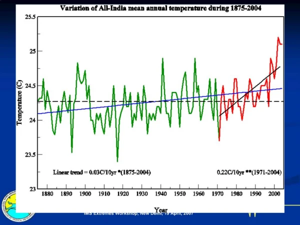
Instrumental Records • First Observatory in Chennai in 1792 • Rainfall/Temperature data network since early 19th century • Century-long rainfall/temperature records for Kathmandu • IITM Homogeneous Monthly Rainfall/Temperature data sets (http://www.tropmet.res.in) • Interannual to Decadal scale variability • All-India/Regional Means • Teleconnection Studies
Proxy Climatic Sources • Historical Records • Tree Rings • Corals • Ice Cores • Lake Sediments • Marine Sediments
REANALYSES • Assimilation of global observational (conventional, satellite, etc.) data archives into atmospheric general circulation models to produce homogeneous and complete data sets describing the state of the atmosphere • Data on daily/monthly scale over resolutions ~ 2° x 2° • NCEP/NCAR Reanalysis (1948 to date) • ECMWF Reanalysis (ERA-15, 1979-93) • ECMWF Reanalysis (ERA-40, 1958-2001) • Useful to validate climate model simulations and also to understand observed climate change and variability on decadal to smaller time scales
Climate Scenarios:What are they ? A climate scenario is a plausible representation of future climate that has been constructed for explicit use in investigating the potential impacts of anthropogenic climate change.
Climate Scenarios:How do we get them ? By using climate projections (description of the modelled response of the climate system to scenarios of greenhouse gas and aerosol concentration), by manipulating the model outputs and combining them with observed climate data.
Types of Climate Scenarios • Climate Model Projections • Incremental Scenarios • Analogue Scenarios • Others
Climate Model Projections • Starting point for most climate scenarios • Simple climate models • General Circulation Models • Large-scale response to anthropogenic forcing • Variety of spatio-temporal resolutions
Special Report on Emission Scenarios (SRES) • A1: Rapid economic growth;Global population peaks in mid-century; Rapid introduction of new and more efficient technologies; Convergence among regions; increased cultural/social interaction; reduction in income disparities • A2: Heterogeneous world; Self-reliance; Preservation of local identities; Continuously increasing population; Regionally oriented economic development; Fragmented per capita economic growth and technological change • B1: Convergent world; Global population peaks in mid-century and declines thereafter; Rapid change in economic structures toward service and information; Reduction in material intensity and introduction of clean/resource-efficient technologies; Global solutions • B2: Local solutions; Continuously increasing population; Intermediate levels of economic development; Less rapid and more diverse technological change; Environmental protection and social equity with focus on local/regional levels.
Incremental Scenarios • Also called synthetic scenarios • Critical climate elements are changed by arbitrary but plausible increments (e.g., +1, +2, +3°C change in temperature) • Testing system sensitivity • Identifying key climate thresholds
Analogue Scenarios • Identifying recorded climate changes that may resemble future climate in a given region • Palaeoclimatic (characterizing warmer periods in the past) • Instrumental (exploring vulnerabilities and adaptive capacities) • Temporal analogues • Spatial analogues
Other Scenarios • Extrapolating observed trends • Statistical downscaling • Expert judgement
Uncertainties in Climate Scenarios • Specifying alternative emissions futures • Uncertainties in converting emissions to concentrations • Uncertainties in converting concentrations to radiative forcing • Uncertainties in modelling the climate response to a given radiative forcing • Uncertainties in converting model response into inputs for impact studies
Approaches for representing uncertainties • Scaling climate response patterns across a range of forcing scenarios • Defining appropriate climate change signals • Risk assessment approaches • Annotation of climate scenarios to reflect more qualitative aspects of uncertainty
Climate Scenarios:Suitability Criteria for Impact Assessment • Consistency • Physical plausibility and Realism • Appropriateness • Representativeness • Accessibility
CLIMATE SCENARIO CONSTRUCTION FOR IMPACT ASSESSMENT NATURAL FORCING (orbital; solar;volcanic) ANTHROPOGENIC FORCING (GHG emissions, land use) Palaeoclimatic reconstructions GCMs Historical Observations Simple Models GCM validation Pattern Scaling GCM present climate Analogue scenarios Baseline Climate Global mean annual temperature change GCM future climate Regionalization Incremental Scenarios For sensitivity studies Dynamical methods Statistical Methods Direct GCM or interpolated GCM based scenarios IMPACTS
Climate Models • Simplified mathematical representation of the Earth’s climate system • Skill depends on the level of our understanding of the physical, geophysical, chemical and biological processes that govern the climate system • Substantial improvements over the last two decades • Sub-models : atmosphere, ocean, land surface, cryosphere, biosphere • Typical Resolution of global models (atmosphere) : Horizontal - 250 km; Vertical – 1 km • Small-scale processes : Parameterization • Coupled models (e.g., atmosphere-ocean) • Sensitivity studies/Future projections • Internal variability/Ensemble runs
Climate Model Projections • Idealized forcing (e.g., 1% compound increase of greenhouse gas concentration extending up to a doubling at year 70) • Time-evolving future forcing, with the simulation starting in the 19th century run with estimates of observed forcing through the 20th century and future climate with estimated forcings according to various scenarios such as IS92a • Using an initial state the end of the 20th century integrations, and following the A2 and B2 SRES forcing scenarios up to 2100
Control (CTL) Carbon Dioxide, Methane and Nitrous Oxide fixed at 1990 levels. Concentrations of the industrial gases (CFCs and others) are set to zero, while ozone and aerosols are prescribed as climatological distributions. ECHAM4/OPYC3: After a 100-year spin-up the model was run, with constant flux adjustment, for another 300 years. HadCM2 and HadCM3: After 510-year spin-up, the model was run for 240 years. Greenhouse Gas Increase (GHG) The GHG simulation starts from the end of the spin-up and the forcing is slowly increased to represent the observed changes in the atmospheric concentration of greenhouse gases during 1860-1990 and during 1990-2099 the forcings are increased at rates specified by the IPCC scenarios (IS92a, 1% per year compounded increase). Greenhouse Gas + Sulfate Aerosol Increase (SUL) The second perturbed experiment involves the forcing due to increasing concentration of greenhouse gases as well as sulfate aerosols. The forcings in this experiment also follow the historical rates during 1860-1990 and the IS92a specifications for the period 1990-2099. The Transient Climate Change Simulations
Model Simulations (Monthly) • (Source: IPCC-DDC and DKRZ, MPI) • Data Period : 240 years (1860-2099; nominal time scale) • Surface Climate variables for three coupled AOGCMs: • ECHAM4/OPYC3,HadCM2 and HadCM3 • Precipitation • Surface Air Temperature (Maximum and Minimum). • Upper air fields for the levels 850, 500 and 200 hPa • (ECHAM4/OPYC3 only) • Winds (u,v) • Temperature • Specific Humidity • Observed Climate (Monthly) • (Source: IMD and others) • Precipitation at 306 stations over India (1871-1990) • Max./Min. Temperatures at 121 stations over India (1901-1990) • Global SST anomalies and Niño-3 SSTA (1856-1997) • Global land surface air temperature anomalies (1856-1999) DATA
Temporal scales of monsoon variability Features Factors
Projected Changes in ENSO-Monsoon Relationshipsdue to Transient increase in Greenhouse Gas Concentrations (ECHAM4/OPYC3)
Regionalization Techniques • High/variable resolution AOGCMs • Regional/nested regional (limited area) climate models • Empirical/statistical downscaling
The Hadley Centre Regional Climate Models(HadRM2/HadRM3) • High-resolution limited area model driven at its lateral and sea-surface boundaries by output from HadCM • Formulation identical to HadAM • Grid : 0.44° x 0.44° • One-way nesting • Joint Indo-UK Collaborative research programme on climate change impacts in India • Climate change simulations performed by the Hadley Centre using HadRM2 for the Indian region (the output is being currently analysed by IITM) • HadRM3 installed at IITM; Climate change simulations and scenario development will be performed at IITM
Observed and Simulated Indian Summer Monsoon Rainfall (GCM vs. RCM)
Observed and Simulated (GCM and RCM) Surface Air Temperature over India
Simulated Surface Temperature Change due to Greenhouse Gas Increase
Simulated Monsoon Rainfall Change (mm/day) due to Greenhouse Gas Increase
Global Summer (JJAS) Precipitation Patterns simulated by 9 coupled AOGCMs
Indian Summer Monsoon Patterns simulated by 9 coupled AOGCMs