Download
1 / 24
240 likes | 383 Views
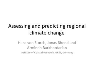
Regional Climate Change. Summary of TAR Findings How well do the Models Work at Regional Scales? Some Preliminary Simulation Results Understanding Climate Variability Versus Scale.

E N D
Regional Climate Change • Summary of TAR Findings • How well do the Models Work at Regional Scales? • Some Preliminary Simulation Results • Understanding Climate Variability Versus Scale
Figure 10.1: Regions used for the analysis presented in Figures 10.2 to 10.5 (from Giorgi and Francisco, 2000b).
Simulations of present day climate Coarse resolution AOGCMs simulate atmospheric general circulation features well in general. At the regional scale the models display area-average biases that are highly variable from region-to-region and among models, with sub-continental area-averaged seasonal temperature biases typically within 4ºC and precipitation biases mostly between -40 and +80% of observations. In most cases, these represent an improvement compared to the AOGCM results evaluated in the SAR. Regional CMs consistently improve the spatial detail of simulated climate compared to General Circulation Models (GCMs). RCMs driven by observed boundary conditions show area-averaged temperature biases (regional scales of 105 to 106 km2) generally within 2ºC and precipitation biases within 50% of observations. Statistical downscaling demonstrates similar performance, although greatly depending on the methodological implementation and application.
Figure 10.2: Surface temperature biases (in °C) for 1961 to 1990 for experiments using the AOGCMs of CSIRO Mk2, CCSR/NIES, ECHAM/OPYC, CGCM1 (a three-member ensemble) and HadCM2 (a four-member ensemble) with historical forcing including sulfates (further experimental details are in Table 9.1). Regions are as indicated in Figure 10.1 and observations are from New et al. (1999a,b). (a) surface air temperature, (b) precipitation (from Giorgi and Francisco, 2000b). Model Bias 1961-1990
Precipitation Model Bias 1961-1990
Spatial Resolution of Global Models 1980s AGCM 1990s AOGCM 2000s AOGCM
Simulation of climate change for the late decades of the 21st century Climate means *It is very likely that: nearly all land areas will warm more rapidly than the global average, particularly those at high latitudes in the cold season; in Alaska, northern Canada, Greenland, northern Asia, and Tibet in winter and central Asia and Tibet in summer the warming will exceed the global mean warming in each model by more than 40% (1.3 to 6.9°C for the range of models and scenarios considered). In contrast, the warming will be less than the global mean in south and Southeast Asia in June-July-August (JJA), and in southern South America in winter. *It is likely that: precipitation will increase over northern mid-latitude regions in winter and over northern high latitude regions and Antarctica in both summer and winter. In December-January-February (DJF), rainfall will increase in tropical Africa, show little change in Southeast Asia and decrease in central America. There will be increase or little change in JJA over South Asia. Precipitation will decrease over Australia in winter and over the Mediterranean region in summer. Change of precipitation will be largest over the high northern latitudes.
Figure 10.3:Simulated temperature changes in °C (mean for 2071 to 2100 minus 1990) conditions of 1%/yr increasing CO2 without and with sulphate forcing using experiments undertaken with the AOGCMs of CSIRO Mk2, CCSR/NIES, ECHAM/OPYC, CGCM1 and Hadley Centre (further experimental details are in Table 9.1). Under both forcing scenarios a four-member ensemble is included of the Hadley Centre model, and under the CO2 plus sulphate scenario a three-member ensemble is included for the CGCM1 model. (a) increased CO2 only (GG), (b) increased CO2 and sulphate aerosols (GS). Global model warming values in the CO2 increase-only experiments are 3.07°C for HadCM2 (ensemble average), 3.06°C for CSIRO Mk2, 4.91°C for CGCM1, 3.00°C for CCSR/NIES and 3.02°C for ECHAM/OPYC. Global model warming values for the experiments including sulphate forcing are 2.52°C for HadCM2 (ensemble average), 2.72°C for CSIRO Mk2, 3.80°C for CGCM1 (ensemble average) and 2.64°C for CCSR/NIES (from Giorgi and Francisco, 2000b). Temperature Changes 2071-2100 from 1990
Figure 10.4: Analysis of inter-model consistency in regional warming relative to each model’s global warming, based on the results presented in Figure 10.3. Regions are classified as showing either agreement on warming in excess of 40% above the global average (“Much greater than average warming”), agreement on warming greater than the global average (“Greater than average warming”), agreement on warming less than the global average (“Less than average warming”), or disagreement amongst models on the magnitude of regional relative warming (“Inconsistent magnitude of warming”). There is also a category for agreement on cooling (which is not used). GG is the greenhouse gas only case (see Figure 10.3a), and, GS, the greenhouse gas with increased sulphate case (see Figure 10.3b). In constructing the figure, ensemble results were averaged to a single case, and “agreement” was defined as having at least four of the five GG models agreeing or three of the four GS models agreeing. The global annual average warming of the models used span 3.0 to 4.9°C for GG and 2.5 to 3.8°C for GS, and therefore a regional 40% amplification represents warming ranges of 4.2 to 6.9°C for GG and 3.5 to 5.3°C for GS.
Figure 10.6: Analysis of inter-model consistency in regional precipitation change based on the results presented in Figure 10.5. Regions are classified as showing either agreement on increase with an average change of greater than 20% (“Large increase”), agreement on increase with an average change between 5 and 20% (“Small increase”), agreement on a change between –5 and +5% or agreement with an average change between –5 and 5% (“No change”), agreement on decrease with an average change between –5 and -20% (“Small decrease”), agreement on decrease with an average change of less than -20% (“Large decrease”), or disagreement (“Inconsistent sign”). GG is the greenhouse gas only case (see Figure 10.5a), and, GS, the greenhouse gas with increased sulphate case (see Figure 10.5b). In constructing the figure, ensemble results were averaged to a single case, and “agreement” was defined as having at least of four the five GG models agreeing or three of the four GS models agreeing.
Figure 10.7: For the European region, simulated change in annual precipitation, averaged by latitude and normalized to % change per °C of global warming. Results are given for twenty-three enhanced GHG simulations (forced by CO2 change only) produced between the years 1983 and 1998. The earlier experiments are those used in the SCENGEN climate scenario generator (Hulme et al., 1995) and include some mixed-layer 1x and 2xCO2 equilibrium experiments; the later ones are the AOGCM experiments available through the DDC. From Hulme et al. (2000).
Climate variability and extremes (1) *Daily to interannual variability of temperature will likely decrease in winter and increase in summer in mid-latitude Northern Hemisphere land areas. *Daily high temperature extremes will likely increase in frequency as a function of the increase in mean temperature, but this increase is modified by changes in daily variability of temperature. There is a corresponding decrease in the frequency of daily low temperature extremes.
Climate variability and extremes (2) *There is a strong correlation between precipitation interannual variability and mean precipitation. Future increases in mean precipitation will very likely lead to increases in variability. Conversely, precipitation variability will likely decrease only in areas of reduced mean precipitation. *For regions where daily precipitation intensities have been analyzed (e.g., Europe, North America, South Asia, Sahel, southern Africa, Australia and the South Pacific) extreme precipitation intensity may increase. *Increases in the occurrence of drought or dry spells are indicated in studies for Europe, North America and Australia.
Tropical cyclones Despite no clear trends in the observations, a series of theoretical and model-based studies, including the use of a high resolution hurricane prediction model, suggest: *It is likely that peak wind intensities will increase by 5 to 10% and mean and peak precipitation intensities by 20 to 30% in some regions; *There is no direct evidence of changes in the frequency or areas of formation.
Just how good is regional modeling? The following simple analysis shows how much of the variance for a small patch on the Earth comes from contributions from very large scales. We use as an example a small patch on a latitude circle. We make a model of fluctuations on the circle and then find how an average on a small patch varies. Then we see how the variability of this patch-average is decomposed into contributions from larger scales on the circle. The finding is that the large scales contribute greatly to the variability of the patch-average. The moral is that it is exceedingly difficult to estimate the variability of a patch-average if we do not have accurate larger scale information.
Consider a Loop such as a Latitude Circle. We can expand the Temperature Anomaly Field into a Fourier Series:
Let’s look at the variance of the average of T from 0 to 0.5
I calculated the Fn for this case Variance of a Small Area Average involves Sum over all scale variances of larger scale
Product of Filter times Spectrum To get the variance of the regional average, sum up the points Note how much variance comes from the larger scales (smaller n)
The Moral: In looking at the variance of a small region. All the variances of Larger scales contribute according to the variance spectrum. The Variance spectrum in geosciences usually is large for large scales (small n) and tapers off for small scales. This makes it very difficult to examine the variability of small scales, because all the larger scales (and their errors) contribute. In terms of regional climate modeling, the implication is that one must have rather accurate large scale information to feed into a high resolution sub-model. (Physically, these are the fluxes in/out) So-called ‘downscaling’ is very difficult.