Download
1 / 10
100 likes | 251 Views
Comparing Means from Paired Samples. (Session 13). Learning Objectives. By the end of this session, you will be able to recognise whether two samples are paired or independent explain why there is a gain in precision with paired samples

E N D
Comparing Means from Paired Samples (Session 13)
Learning Objectives By the end of this session, you will be able to • recognise whether two samples are paired or independent • explain why there is a gain in precision with paired samples • carry out a paired t-test and interpret results from such a test • present and report on conclusions from paired t-tests
Paired samples - aims In comparing two samples we would aim to improve the precision of the comparison wherever possible, i.e. reduce the standard error used in the test statistic. e.g. If the aim is to compare the average weight of males with that of females amongst malnourished children, it would be better to assess pairs of children of the same age, having one male and one female in each pair.
Benefits of pairing The paired approach means that gender difference would be clearer within a pair of the same age, thus removing age to age variability from the comparison. The situation could be further improved by matching the children, not only by age, but other characteristics too, e.g. their location (rural or urban), levels of poverty, etc. Matching leads to a study of the differences between each pair, say di for pair i.
An example Suppose we have data for the mean annual income (in 1000’s), of doctors and dentists in the UK, from 10 different regions. The data (fictitious) are given in the table.
Null and alternative hypotheses The hypotheses to be tested are: H0:1 - 2 = 0 versus H1:1 - 2 0 This is equivalent to H0:d = 0 versus H1:d 0 where d refers the mean of the population of differences between the two groups. Thus, the two-sample case reduces to a single sample situation. Hence ideas covered in Session 09 applies to the single sample formed from differences between each set of pairs.
Test procedure The ten differences are found to be: -0.7 0.6 0.6 2.1 2.6 2.4 1.4 0.9 2.7 -0.4 Further, = 1.22, while = 1.497 Hence the t-statistic for testing H0 is: t = = = 3.15 Comparing with t-tables with 9 d.f. shows this result is significant at the 2% significance level. The exact p-value = 0.012
Conclusions and other issues Conclusion: There is some evidence of a difference between the mean salaries at a 2% significance level. Note: If we had ignored the pairing by region and conducted an independent samples (or two-sample t-test), the test statistic is t= 1.95 on 18 d.f. This is clearly non-significant, thus leading to a different conclusion from above. So take care to recognise pairing where it occurs.
References Armitage, P., Matthews J.N.S. and Berry G. (2002). Statistical Methods in Medical Research. 4th edn. Blackwell. Clarke, G.M. and Cooke, D. (2004). A Basic Course in Statistics. 5th edn. Edward Arnold. Johnson, R.A. and Bhattacharyya, G.K. (2001). Statistics Principles and Methods. 4th edn. Wiley.