Download
1 / 60
610 likes | 1.04k Views
Inference for Means. CH23 And Ch 24&25. Quantitative Data. The population of interest has a certain mean μ we want to estimate. Gather a representative sample get a an estimate for the true mean the sample mean:

E N D
Inference for Means CH23 And Ch 24&25
Quantitative Data The population of interest has a certain mean μwe want to estimate. Gather a representative sample • get a an estimate for the true mean the sample mean: This estimate is just a single number so it is referred to as a “point estimate”.
Population of interest Population has mean μ Sample of size n y¯=115 Estimate for μ
Sample Mean The mean of the sample mean: The standard deviation of the sample mean:
Note for the curious: • Each observation comes from the same distribution, so it has a mean of μ and a standard deviation σ. Observations are independent. Mean Variance: Thus:
Normal Model again • The Central Limit Theorem tells us that the distribution of the sample mean y¯ is approximately normal, with mean μ and standard deviation σ/sqrt(n). • This is very helpful to: • Find probabilities • Construct confidence intervals • Run test of hypothesis
When can I use the normal model? Either n is large Or the original population distribution is normal (in this case, the distribution of the sample mean is also normal)
Confidence Intervals Since we are using the normal model, then The z-score of the sample mean is approximately a standard normal:
So, if we proceed like we did for proportions, we would get a similar formula for confidence interval:
Confidence Intervals But what happens if we do not know σ?
But what happens if we do not know σ? • We estimate the standard deviation • by the standard error:
The T-distribution When the conditions are met, the standardized sample mean follows a Student’s t-model with n – 1 degrees of freedom.
The t-distribution vs the standard normal • T-distribution normal as n goes to infinity
Which of the following is true about • Student’s t-models? • They are unimodal, symmetric, and bell shaped. • They have fatter tails than the Normal model. • As the degrees of freedom increase, the t-models look more and more like the Normal Model • All of the above.
Which of the following is true about • Student’s t-models? • They are unimodal, symmetric, and bell shaped. • They have fatter tails than the Normal model. • As the degrees of freedom increase, the t-models look more and more like the Normal Model • All of the above.
Confidence Intervals for the mean Confidence multiplier (critical value) For the t-distribution with (n-1) df
Confidence Interval for Means From here on, we will use the formula with the SE:
Finding t-Values By Hand • The Student’s t-model is different for each value of degrees of freedom.
T-table one tail normal
Ex: The mean hours slept (per day) among a sample (of size 20) of college students was 7.1, with a standard deviation of 1.65. Construct a 90% CI for the mean hours of sleep college students get.
Are conditions for inference met? That is ,can we apply the normal model? We can assume the sample was random. The sample size n=20, is not large. So we need to think if it is reasonable to assume the distribution of hors of sleep is normal. It might change during exam times, but on regular days it is close to normal. T-table
Point estimates: y¯=7.1, s=1.65 df=n-1=19 t*= 1.729 Margin of error: t* s/sqrt(n) =(1.729)(1.65)/sqrt(20)=.64 CI: 7.1 ± .64 which gives (6.46,7.74) Interpretation: we are 90% sure that the average number of hours of sleep college students get is between 6.46 and 7.74 hours.
A professor was curious about her students’ grade point averages (GPAs). She took a random sample of 15 students and found a mean GPA of 3.01 with a standard deviation of 0.534. Which of the following formulas gives a 99% confidence interval for the mean GPA of the professor’s students? T-table
A professor was curious about her students’ grade point averages (GPAs). She took a random sample of 15 students and found a mean GPA of 3.01 with a standard deviation of 0.534. Which of the following formulas gives a 99% confidence interval for the mean GPA of the professor’s students?
A researcher found that a 98% confidence interval • for the mean hours per week spent studying by • college students was (13, 17). Which is true? • There is a 98% chance that the mean hours per week spent studying by college students is between 13 and 17 hours. • We are 98% sure that the mean hours per week spent studying by college students is between 13 and 17 hours. • Students average between 13 and 17 hours per week studying on 98% of the weeks. • 98% of all students spend between 13 and 17 hours studying per week.
A researcher found that a 98% confidence interval • for the mean hours per week spent studying by • college students was (13, 17). Which is true? • There is a 98% chance that the mean hours per week spent studying by college students is between 13 and 17 hours. • We are 98% sure that the mean hours per week spent studying by college students is between 13 and 17 hours. • Students average between 13 and 17 hours per week studying on 98% of the weeks. • 98% of all students spend between 13 and 17 hours studying per week.
Suppose that based on a random sample, a 95% confidence interval for the mean hours slept (per day) among graduate students was found to be (6.5, 6.9). What is the margin of error of this confidence interval? Length of interval: 6.9-6.5=.4 Margin of error: m=1/2 of length = .4/2=.2
Test of Hypothesis for a Mean Step 1: Assumptions (normal model -> nearly normal condition + independence) Step 2: Hypothesis Ho: μ=μo vs one of these alsternatives Ha: μ>μo Ha: μ<μo Ha: μμo Step 3: Test statistic (T-test) Step 4: p-value Step 5: Conclusion
Assumptions When doing Confidence Intervals or Test of Hypothesis for means, we need to check the NEARLY NORMAL condition: • Either the original distribution is normal or • Sample size is big enough (so the central Limit Theorem applies)
EX: Researchers tested 150 farmed raised salmon for organic contaminants. The found the mean concentration of carcinogenic insecticide mirex to be 0.0913 parts per million, with as standard deviation of 0.0495. The EPA recommends a safety level for mirex of 0.08 ppm. Are farmed salmon contaminated beyond the level permitted by the EPA?
What we know: y¯=.0913, s=.0495, n=150 • Assumptions: sample was random, n is large enough so nearly normal condition is satisfied. (10% condition is also satisfied). • Ho: μ=0.08 (EPA safety level) • Ha: μ>0.08 (contaminated) • Test stat: t=(y¯- μo)/SE df=n-1 SE=s/sqrt(n)=0.0495/sqrt(150)=0.004042 t=(0.0913-0.08)/0.004=2.825
P-value: recall the alternative: Ha: μ>0.08 The p-value is P(T>2.825) Where T is the t-distribution with df=149. Using a statistical software, I get P(T>2.825)=0.002688 • Conclusion: there is strong statistical evidence at the 5% level that farmed salmon are contaminated with mirex beyond the level permitted by the EPA.
EX: Students investigating the packaging of potato chips purchased 6bags of Lay’s Ruffles marked with a net weight of 28.3 g. They recorded the weights:29.3, 28.2, 29.1, 28.7, 28.9, 28.5
Assumptions: distribution comes from a machine probably normal Find a 95% CI for mean weight: • Sample mean: 28.78 • Sample standard deviation: s=0.4 • SE=s/sqrt(n)=0.4/sqrt(6)=.16 • df=n-1=5 t=2.571 • Margin of error: m=(2.571)(.16)=.41 • CI: 28.78±.41 (28.37,29.19) • We are 95% sure that the average Lay’s Ruffles 28.3g bag contains between 38.37g and 29.19g. • This provides evidence supporting the company’s claim that the bags contain at least 28.3g.
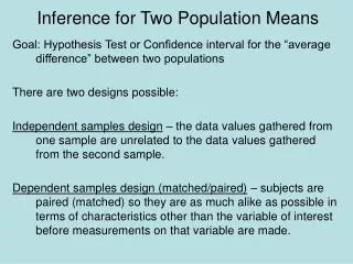
Comparing Means of 2 Groups Are the groups independent??? Independent 2-sample T-test Paired paired T-test
Ex: Does Ginkgo Bilboa enhance memory? Subjects were randomly assigned to take ginkgo bilboa or a placebo. Their memory was tested to see whether it improved. We have 2 independent groups: • The group of people taking ginkgo bilboa • The placebo group
Ex: Many dairy cows receive injections of BST. After the first injection, a test of 60 Ayrshyre cows increased their mean daily production from 47 pounds to 61 pounds of milk. Estimate the mean increase. Here there are also 2 groups: (a) measurements before the injection of BST (b) measurement after BST. The groups are dependent. The measurement were done on the same cows (before and after).
The natural display for comparing two groups is boxplots of the data for the two groups, placed side-by-side. For example: Comparing 2 groups: Plot the Data
Comparing Two Independentgroups Means: μ1- μ2 • Remember that, for independent random quantities, variances add. standard deviation of the difference • We use the standard error to estimate SD
Comparing 2 (independent groups) means • The confidence interval we build is called a two-sample t-interval(for the difference in means). • The corresponding hypothesis test is called a two-sample t-test.
Sampling Distribution for the Difference Between Two Means • Statistic use: if assumptions are met, it can be modeled by a Student’s t-model with a number of degrees of freedom found with a special formula.
Two-Sample t-Interval(independent groups) The confidence interval is where the standard error of the difference of the means is the degrees of freedom has a complicated formula.
Degrees of Freedom • The special formula for the degrees of freedom for our t critical value is a bear: • Because of this, we will let technology calculate degrees of freedom for us!
A Test for the Difference Between Two Means We test the hypothesis H0: 1 – 2 = 0, (usually 0=0), using the statistic The standard error is
Ex: Below you'll find three sample outputs of the two-sided two-sample t-test However, only one of the outputs could be correct (the other two contain an inconsistency). Your task is to decide which of the following outputs is the correct one (Hint: No calculations are necessary in order to answer this question. Instead pay attention to the p-value and confidence interval). • Output A: p-value: 0.289 95% CI: (-5.93090, -1.78572) • Output B: p-value: 0.003 95% CI: (-13.97384, 2.89733) • Output C: p-value: 0.223 95% CI: (-9.31432, 2.20505)
Ex: Below you'll find three sample outputs of the two-sided two-sample t-test However, only one of the outputs could be correct (the other two contain an inconsistency). Your task is to decide which of the following outputs is the correct one (Hint: No calculations are necessary in order to answer this question. Instead pay attention to the p-value and confidence interval). • Output A: p-value: 0.289 95% CI: (-5.93090, -1.78572) • Output B: p-value: 0.003 95% CI: (-13.97384, 2.89733) • Output C: p-value: 0.223 95% CI: (-9.31432, 2.20505)
When groups are dependent: A Paired t-Test • Responses are “paired”: • Take their difference: • We test the hypothesis H0: d = 0, where the d’s are the pairwise differences and 0 is almost always 0. d = average mean of the differences= 1 - 2 But we want to emphasize that the test is run using differences.
A Paired t-Test (cont.) The paired t-test • We use the statistic where is the mean of the pairwise differences and n is the number of pairs. • is the ordinary standard error for the mean, applied to the differences: • Note: d¯= x¯-y¯