Download
1 / 21
210 likes | 332 Views
CSC321 Lecture 24 Using Boltzmann machines to initialize backpropagation . Geoffrey Hinton. Some problems with backpropagation. The amount of information that each training case provides about the weights is at most the log of the number of possible output labels.

E N D
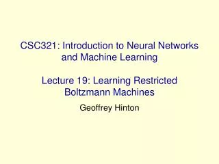
CSC321 Lecture 24Using Boltzmann machines to initialize backpropagation Geoffrey Hinton
Some problems with backpropagation • The amount of information that each training case provides about the weights is at most the log of the number of possible output labels. • So to train a big net we need lots of labeled data. • In nets with many layers of weights the backpropagated derivatives either grow or shrink multiplicatively at each layer. • Learning is tricky either way. • Dumb gradient descent is not a good way to perform a global search for a good region of a very large, very non-linear space. • So deep nets trained by backpropagation are rare in practice.
A solution to all of these problems • Use greedy unsupervised learning to find a sensible set of weights one layer at a time. Then fine-tune with backpropagation. • Greedily learning one layer at a time scales well to really deep networks. • Most of the information in the final weights comes from modeling the distribution of input vectors. • The precious information in the labels is only used for the final fine-tuning. • We do not start backpropagation until we already have sensible weights that already do well at the task. • So the fine-tuning is well-behaved and quite fast.
Modelling the distribution of digit images The top two layers form a restricted Boltzmann machine whose free energy landscape should model the low dimensional manifolds of the digits. 2000 units 500 units The network learns a density model for unlabeled digit images. When we generate from the model we often get things that look like real digits of all classes. More hidden layers make the generated fantasies look better (YW Teh, Simon Osindero). But do the hidden features really help with digit discrimination? Add 10 softmaxed units to the top and do backprop. 500 units 28 x 28 pixel image
Results on permutation-invariant MNIST task • Very carefully trained backprop net with 1.53% one or two hidden layers (Platt; Hinton) • SVM (Decoste & Schoelkopf) 1.4% • Generative model of joint density of 1.25% images and labels (with unsupervised fine-tuning) • Generative model of unlabelled digits 1.2% followed by gentle backpropagtion • Generative model of joint density 1.1% followed by gentle backpropagation
Why does greedy learning work? The weights, W, in the bottom level RBM define p(v|h) and they also, indirectly, define p(h). So we can express the RBM model as If we leave p(v|h) alone and build a better model of p(h), we will improve p(v). We need a better model of the posterior hidden vectors produced by applying W to the data.
Deep Autoencoders • They always looked like a really nice way to do non-linear dimensionality reduction: • They provide mappings both ways • The learning time is linear (or better) in the number of training cases. • The final model is compact and fast. • But it turned out to be very very difficult to optimize deep autoencoders using backprop. • We now have a much better way to optimize them.
The deep autoencoder 784 1000 500 250 30 linear units 784 1000 500 250 If you start with small random weights it will not learn. If you break symmetry randomly by using bigger weights, it will not find a good solution. So we train a stack of 4 RBM’s and then “unroll” them. Then we fine-tune with gentle backprop.
A comparison of methods for compressing digit images to 30 real numbers. real data 30-D deep auto 30-D logistic PCA 30-D PCA
A very deep autoencoder for synthetic curves that only have 6 degrees of freedom squared error Data 0.0 Auto:6 1.5 PCA:6 10.3 PCA:30 3.9
An autoencoder for patches of real faces • 6252000100064130 and back out again linear linear logistic units Train on 100,000 denormalized face patches from 300 images of 30 people. Use 100 epochs of CD at each layer followed by backprop through the unfolded autoencoder. Test on face patches from 100 images of 10 new people.
Reconstructions of face patches from new people Data Auto:30 126 PCA:30 135
How to find documents that are similar to a query document • Convert each document into a “bag of words”. • This is a vector of word counts ignoring the order. • Ignore stop words (like “the” or “over”) • We could compare the word counts of the query document and millions of other documents but this is too slow. • So we reduce each query vector to a much smaller vector that still contains most of the information about the content of the document. fishcheese vector count school query reduce bag pulpit iraq word 0 0 2 2 0 2 1 1 0 0 2
We train the neural network to reproduce its input vector as its output This forces it to compress as much information as possible into the 10 numbers in the central bottleneck. These 10 numbers are then a good way to compare documents. How to compress the count vector output vector 2000 reconstructed counts 500 neurons 250 neurons 10 250 neurons 500 neurons input vector 2000 word counts
The non-linearity used for reconstructing bags of words • Divide the counts in a bag of words vector by N, where N is the total number of non-stop words in the document. • The resulting probability vector gives the probability of getting a particular word if we pick a non-stop word at random from the document. • At the output of the autoencoder, we use a softmax. • The probability vector defines the desired outputs of the softmax. • When we train the first RBM in the stack we use the same trick. • We treat the word counts as probabilities, but we make the visible to hidden weights N times bigger than the hidden to visible because we have N observations from the probability distribution.
Performance of the autoencoder at document retrieval • Train on bags of 2000 words for 400,000 training cases of business documents. • First train a stack of RBM’s. Then fine-tune with backprop. • Test on a separate 400,000 documents. • Pick one test document as a query. Rank order all the other test documents by using the cosine of the angle between codes. • Repeat this using each of the 400,000 test documents as the query (requires 0.16 trillion comparisons). • Plot the number of retrieved documents against the proportion that are in the same hand-labeled class as the query document. Compare with LSA (a version of PCA).
Proportion of retrieved documents in same class as query Number of documents retrieved
First compress all documents to 2 numbers using a type of PCA Then use different colors for different document categories
First compress all documents to 2 numbers. Then use different colors for different document categories