Backpropagation

1. Backpropagation CS 478 – Backpropagation

2. CS 478 – Backpropagation

3. CS 478 – Backpropagation

4. CS 478 – Backpropagation

5. Backpropagation • Rumelhart (early 80’s), Werbos (74),…, explosion of neural net interest • Multi-layer supervised learning • Able to train multi-layer perceptrons (and other topologies) • Uses differentiable sigmoid function which is the smooth (squashed) version of the threshold function • Error is propagated back through earlier layers of the network CS 478 – Backpropagation

6. Multi-layer Perceptrons trained with BP • Can compute arbitrary mappings • Training algorithm less obvious • First of many powerful multi-layer learning algorithms CS 478 – Backpropagation

7. Responsibility Problem Output 1 Wanted 0 CS 478 – Backpropagation

8. Multi-Layer Generalization CS 478 – Backpropagation

9. Multilayer nets are universal function approximators • Input, output, and arbitrary number of hidden layers • 1 hidden layer sufficient for DNF representation of any Boolean function - One hidden node per positive conjunct, output node set to the “Or” function • 2 hidden layers allow arbitrary number of labeled clusters • 1 hidden layer sufficient to approximate all bounded continuous functions • 1 hidden layer the most common in practice CS 478 – Backpropagation

10. CS 478 – Backpropagation

11. Backpropagation • Multi-layer supervised learner • Gradient descent weight updates • Sigmoid activation function (smoothed threshold logic) • Backpropagation requires a differentiable activation function CS 478 – Backpropagation

12. 1 0 .99 .01 CS 478 – Backpropagation

13. Multi-layer Perceptron (MLP) Topology Input Layer Hidden Layer(s) Output Layer CS 478 – Backpropagation

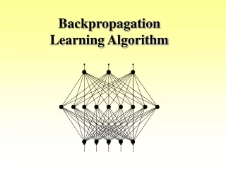
14. Backpropagation Learning Algorithm • Until Convergence (low error or other stopping criteria) do • Present a training pattern • Calculate the error of the output nodes (based on T - Z) • Calculate the error of the hidden nodes (based on the error of the output nodes which is propagated back to the hidden nodes) • Continue propagating error back until the input layer is reached • Update all weights based on the standard delta rule with the appropriate error function d Dwij = C djZi CS 478 – Backpropagation

15. Activation Function and its Derivative • Node activation function f(net) is typically the sigmoid • Derivative of activation function is a critical part of the algorithm 1 .5 0 -5 0 5 Net .25 0 -5 5 0 Net CS 478 – Backpropagation

16. i k i j k i k i Backpropagation Learning Equations CS 478 – Backpropagation

17. CS 478 – Backpropagation

18. CS 478 – Backpropagation

19. CS 478 – Backpropagation

20. CS 478 – Backpropagation

21. Inductive Bias & Intuition • Node Saturation - Avoid early, but all right later • When saturated, an incorrect output node will still have low error • Start with weights close to 0 • Saturated error even when wrong? – Multiple TSS drops • Not exactly 0 weights (can get stuck), random small Gaussian with 0 mean • Can train with target/error deltas (e.g. .1 and .9 instead of 0 and 1) • Intuition • Manager approach • Gives some stability • Inductive Bias • Start with simple net (small weights, initially linear changes) • Smoothly build a more complex surface until stopping criteria CS 478 – Backpropagation

22. Multi-layer Perceptron (MLP) Topology Input Layer Hidden Layer(s) Output Layer CS 478 – Backpropagation

23. Local Minima • Most algorithms which have difficulties with simple tasks get much worse with more complex tasks • Good news with MLPs • Many dimensions make for many descent options • Local minima more common with very simple/toy problems, very rare with larger problems and larger nets • Even if there are occasional minima problems, could simply train multiple nets and pick the best • Some algorithms add noise to the updates to escape minima CS 478 – Backpropagation

24. Local Minima and Neural Networks • Neural Network can get stuck in local minima for small networks, but for most large networks (many weights), local minima rarely occur in practice • This is because with so many dimensions of weights it is unlikely that we are in a minima in every dimension simultaneously – almost always a way down CS 312 – Approximation

25. Batch Update • With On-line (stochastic) update we update weights after every pattern • With Batch update we accumulate the changes for each weight, but do not update them until the end of each epoch • Batch update gives a correct direction of the gradient for the entire data set, while on-line could do some weight updates in directions quite different from the average gradient of the entire data set • Based on noisy instances and also just that specific instances will not represent the average gradient • Proper approach? - Conference experience • Most (including us) assumed batch more appropriate, but batch/on-line a non-critical decision with similar results • We show that batch is less efficient – more in 678 CS 478 – Backpropagation

26. Learning Rate Learning Rate - Relatively small (.1 - .5 common), if too large BP will not converge or be less accurate, if too small is slower with no accuracy improvement as it gets even smaller Gradient – only where you are, too big of jumps? CS 478 – Backpropagation

27. Momentum • Simple speed-up modification w(t+1) = C xi + w(t) • Weight update maintains momentum in the direction it has been going • Faster in flats • Could leap past minima (good or bad) • Significant speed-up, common value ≈ .9 • Effectively increases learning rate in areas where the gradient is consistently the same sign. (Which is a common approach in adaptive learning rate methods). • These types of terms make the algorithm less pure in terms of gradient descent. However • Not a big issue in overcoming local minima • Not a big issue in entering bad local minima CS 478 – Backpropagation

28. Learning Parameters • Momentum – (.5 … .99) • Connectivity: typically fully connected between layers • Number of hidden nodes: too many nodes make learning slower, could overfit (but usually OK if using a reasonable stopping criteria), too few can underfit • Number of layers: usually 1 or 2 hidden layers which seem to be sufficient, attenuation makes learning very slow – 1 most common • Most common method to set parameters: a few trial and error runs • All of these could be set automatically by the learning algorithm and there are numerous approaches to do so CS 478 – Backpropagation

29. Stopping Criteria and Overfit Avoidance SSE • More Training Data (vs. overtraining - One epoch limit) • Validation Set - save weights which do best job so far on the validation set. Keep training for enough epochs to be fairly sure that no more improvement will occur (e.g. once you have trained m epochs with no further improvement, stop and use the best weights so far, or retrain with all data). • Note: If using N-way CV with a validation set, do n runs with 1 of n data partitions as a validation set. Save the number i of training epochs for each run. To get a final model you can train on all the data and stop after the average number of epochs, or a little less than the average since there is more data. • Specific techniques for avoiding overfit • Less hidden nodes, Weight decay, Pruning, Jitter, Regularization, Error deltas Validation/Test Set Training Set Epochs CS 478 – Backpropagation

30. Validation Set - ML Manager • Often you will use a validation set (separate from the training or test set) for stopping criteria, etc. • In these cases you should take the validation set out of the training set which has already been allocated by the ML manager. • For example, you might use the random test set method to randomly break the original data set into 80% training set and 20% test set. Independent and subsequent to the above routines you would take n% of the training set to be a validation set for that particular training exercise. CS 478 - Backpropagation

31. Multiple Outputs • Typical to have multiple output nodes, even with just one output feature (e.g. Iris data set) • Would if there are multiple "independent output features" • Could train independent networks • Also common to have them share hidden layer • May find shared features • Transfer Learning • Could have shared and separate subsequent hidden layers, etc. • Structured Outputs • Multiple Output Dependency? (MOD) • New research area CS 478 – Backpropagation

32. Debugging your ML algorithms • Project http://axon.cs.byu.edu/~martinez/classes/478/Assignments.html • Do a small example by hand and make sure your algorithm gets the exact same results • Compare results with supplied snippets from our website • Compare results (not code, etc.) with classmates • Compare results with a published version of the algorithms (e.g. WEKA), won’t be exact because of different training/test splits, etc. • Use Zarndt’s thesis (or other publications) to get a ballpark feel of how well you should expect to do on different data sets. http://axon.cs.byu.edu/papers/Zarndt.thesis95.pdf

33. Localist vs. Distributed Representations • Is Memory Localist (“grandmother cell”) or distributed • Output Nodes • One node for each class (classification) • One or more graded nodes (classification or regression) • Distributed representation • Input Nodes • Normalize real and ordered inputs • Nominal Inputs - Same options as above for output nodes • Hidden nodes - Can potentially extract rules if localist representations are discovered. Difficult to pinpoint and interpret distributed representations. CS 478 – Backpropagation

34. Hidden Nodes • Typically one fully connected hidden layer. Common initial number is 2n or 2logn hidden nodes where n is the number of inputs • In practice train with a small number of hidden nodes, then keep doubling, etc. until no more significant improvement on test sets • All output and hidden nodes should have bias weights • Hidden nodes discover new higher order features which are fed into the output layer • Zipser - Linguistics • Compression CS 478 – Backpropagation

35. Application Example - NetTalk • One of first application attempts • Train a neural network to read English aloud • Input Layer - Localist representation of letters and punctuation • Output layer - Distributed representation of phonemes • 120 hidden units: 98% correct pronunciation • Note steady progression from simple to more complex sounds CS 478 – Backpropagation

36. Batch Update • With On-line (stochastic) update we update weights after every pattern • With Batch update we accumulate the changes for each weight, but do not update them until the end of each epoch • Batch update gives a correct direction of the gradient for the entire data set, while on-line could do some weight updates in directions quite different from the average gradient of the entire data set • Based on noisy instances and also just that specific instances will not represent the average gradient • Proper approach? - Conference experience • Most (including us) assumed batch more appropriate, but batch/on-line a non-critical decision with similar results • We tried to speed up learning through "batch parallelism" CS 478 – Backpropagation

37. On-Line vs. Batch Wilson, D. R. and Martinez, T. R., The General Inefficiency of Batch Training for Gradient Descent Learning, Neural Networks, vol. 16, no. 10, pp. 1429-1452, 2003 • Many people still not aware of this issue - Changing • Misconception regarding “Fairness” in testing batch vs. on-line with the same learning rate • BP already sensitive to LR - why? • With batch need a smaller LR (/n) since weight changes accumulate • To be "fair", on-line should have a comparable LR?? • Initially tested on relatively small data sets • On-line update approximately follows the curve of the gradient as the epoch progresses • For small enough learning rate batch gives correct result, just less efficient CS 478 – Backpropagation

38. CS 478 – Backpropagation

39. CS 478 – Backpropagation

40. CS 478 – Backpropagation

41. CS 478 – Backpropagation

42. CS 478 – Backpropagation

43. Semi-Batch on Digits CS 478 – Backpropagation

44. On-Line vs. Batch Issues • Some say just use on-line LR but divide by n (training set size) to get the same feasible LR for both (non-accumulated), but on-line still does n times as many updates per epoch as batch and is thus much faster • True Gradient - We just have the gradient of the training set anyways which is an approximation to the true gradient and true minima • Momentum and true gradient - same issue with other enhancements such as adaptive LR, etc. • Training sets are getting larger - makes discrepancy worse since we would do batch update relatively less often • Large training sets great for learning and avoiding overfit - best case scenario is huge/infinite set where never have to repeat - just 1 partial epoch and just finish when learning stabilizes – batch in this case? • Still difficult to convince some people CS 478 – Backpropagation

45. Adaptive Learning Rate/Momentum • Momentum is a simple speed-up modification w(t+1) = C xi + w(t) • Are we true gradient descent when using this? • Weight update maintains momentum in the direction it has been going • Faster in flats • Could leap past minima (good or bad), but not a big issue in practice • Significant speed-up, common value ≈ .9 • Effectively increases learning rate in areas where the gradient is consistently the same sign. • Adaptive Learning rate methods • Start LR small • As long as weight change is in the same direction, increase a bit (e.g. scalar multiply > 1, etc.) • If weight change changes directions (i.e. sign change) reset LR to small, could also backtrack for that step, or … CS 478 – Backpropagation

46. Learning Variations • Different activation functions - need only be differentiable • Different objective functions • Cross-Entropy • Classification Based Learning • Higher Order Algorithms - 2nd derivatives (Hessian Matrix) • Quickprop • Conjugate Gradient • Newton Methods • Constructive Networks • Cascade Correlation • DMP (Dynamic Multi-layer Perceptrons) CS 478 – Backpropagation

47. Classification Based (CB) Learning Target Actual BP Error CB Error 1 .6 .4*f '(net) 0 0 .4 -.4*f '(net) 0 0 .3 -.3*f '(net) 0 CS 478 – Backpropagation

48. Classification Based Errors Target Actual BP Error CB Error 1 .6 .4*f '(net) .1 0 .7 -.7*f '(net) -.1 0 .3 -.3*f '(net) 0 CS 478 – Backpropagation

49. Results • Standard BP: 97.8% Sample Output: CS 478 – Backpropagation

50. Results • Classification Based Training: 99.1% Sample Output: CS 478 – Backpropagation