Download

1 / 47
470 likes | 581 Views
Boltzmann Machines and their Extensions. S. M. Ali Eslami Nicolas Heess John Winn. March 2013 Heriott -Watt University. Goal. Define a probabilistic distribution on images like this:. What can one do with an ideal shape model?. Segmentation. Weizmann horse dataset.

E N D
Boltzmann Machines and their Extensions S. M. Ali Eslami Nicolas Heess John Winn March 2013 Heriott-Watt University
Goal Define a probabilistic distribution on images like this:
What can one do with an ideal shape model? Segmentation
Weizmann horse dataset Sample training images 327 images
What can one do with an ideal shape model? Computer graphics
Energy based models Gibbs distribution
Existing shape models Most commonly used architectures Mean MRF sample from the model sample from the model
What is a strong model of shape? We define a strong model of object shape as one which meets two requirements: Realism Generalization Generates samples that look realistic Can generate samples that differ from training images Training images Real distribution Learned distribution
Shallow architectures HOP-MRF
Shallow architectures Restricted Boltzmann Machines The effect of the latent variables can be appreciated by considering the marginal distribution over the visible units:
Shallow architectures Restricted Boltzmann Machines In fact, the hidden units can be summed out analytically. The energy of this marginal distribution is given by: where
Shallow architectures Restricted Boltzmann Machines All hidden units are conditionally independent given the visible units and vice versa.
RBM inference Block-Gibbs MCMC
RBM inference Block-Gibbs MCMC
RBM learning Stochastic gradient descent Maximize with respect to
RBM learning Contrastive divergence Getting an unbiased sample of the second term, however is very difficult. It can be done by starting at any random state of the visible units and performing Gibbs sampling for a very long time. Instead:
RBM inference Block-Gibbs MCMC
RBM inference Block-Gibbs MCMC
RBM learning Contrastive divergence • Crudely approximating the gradient of the log probability of the training data. • More closely approximating the gradient of another objective function called the Contrastive Divergence, but it ignores one tricky term in this objective function so it is not even following that gradient. • Sutskeverand Tieleman have shown that it is not following the gradient of anyfunction. • Nevertheless, it works well enough to achieve success in many significant applications.
Deep architectures Deep Boltzmann Machines
Deep architectures Deep Boltzmann Machines Conditional distributions remain factorised due to layering.
Shallow and Deep architectures Modeling high-order and long-range interactions MRF RBM DBM
Deep Boltzmann Machines • Probabilistic • Generative • Powerful Typically trained with many examples. We only have datasets with few training examples. DBM
From the DBM to the ShapeBM Restricted connectivity and sharing of weights Limited training data, therefore reduce the number of parameters: • Restrict connectivity, • Tie parameters, • Restrict capacity. DBM ShapeBM
Shape Boltzmann Machine Architecture in 2D Top hidden units capture object pose Given the top units, middle hidden units capture local (part) variability Overlap helps prevent discontinuities at patch boundaries
ShapeBM inference Block-Gibbs MCMC image reconstruction sample 1 sample n Fast: ~500 samples per second
ShapeBM learning Stochastic gradient descent Maximize with respect to • Pre-training • Greedy, layer-by-layer, bottom-up, • ‘Persistent CD’ MCMC approximation to the gradients. • Joint training • Variational + persistent chain approximations to the gradients, • Separates learning of local and global shape properties. ~2-6 hours on the small datasets that we consider
Sampled shapes Evaluating the Realism criterion Weizmann horses – 327 images Weizmann horses – 327 images – 2000+100 hidden units Data Incorrect generalization FA Failure to learn variability RBM Natural shapes Variety of poses Sharply defined details Correct number of legs (!) ShapeBM
Sampled shapes Evaluating the Realism criterion Weizmann horses – 327 images Weizmann horses – 327 images – 2000+100 hidden units This is great, but has it just overfit?
Sampled shapes Evaluating the Generalization criterion Weizmann horses – 327 images – 2000+100 hidden units Sample from the ShapeBM Closest image in training dataset Difference between the two images
Interactive GUI Evaluating Realism and Generalization Weizmann horses – 327 images – 2000+100 hidden units
Further results Sampling and completion Caltech motorbikes – 798 images – 1200+50 hidden units Training images ShapeBM samples Sample generalization Shape completion
Constrained shape completion Evaluating Realism and Generalization Weizmann horses – 327 images – 2000+100 hidden units NN ShapeBM
Further results Constrained completion Caltech motorbikes – 798 images – 1200+50 hidden units NN ShapeBM
Imputation scores Quantitative comparison Weizmann horses – 327 images – 2000+100 hidden units • Collect 25 unseen horse silhouettes, • Divide each into 9 segments, • Estimate the conditional log probability of a segment under the model given the rest of the image, • Average over images and segments.
Multiple object categories Simultaneous detection and completion Caltech-101 objects – 531 images – 2000+400 hidden units Train jointly on 4 categories without knowledge of class: Shape completion Sampled shapes
What does h2do? Weizmann horses Pose information Multiple categories Class label information Accuracy Number of training images
Summary • Shape models are essential in applications such as segmentation, detection, in-painting and graphics. • The ShapeBM characterizes a strong model of shape: • Samples are realistic, • Samples generalize from training data. • The ShapeBM learns distributions that are qualitatively and quantitatively better than other models for this task.
Questions MATLAB GUI available at http://arkitus.com/Ali/