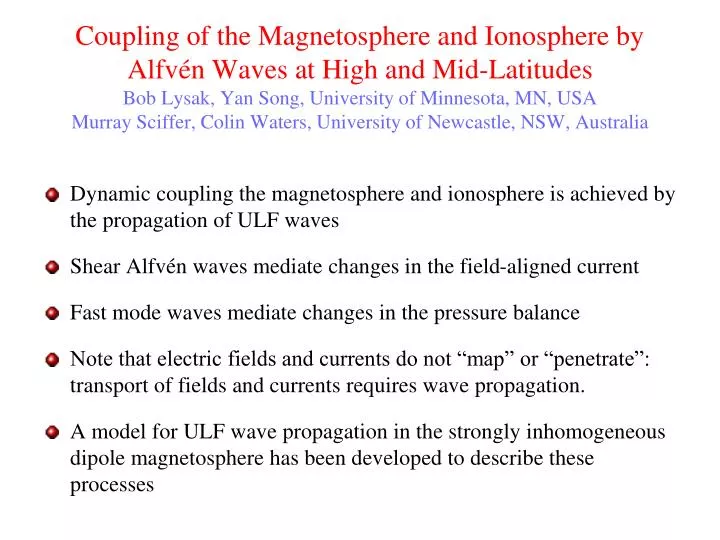
Dynamic coupling the magnetosphere and ionosphere is achieved by the propagation of ULF waves

1. Coupling of the Magnetosphere and Ionosphere by Alfvén Waves at High and Mid-LatitudesBob Lysak, Yan Song, University of Minnesota, MN, USAMurray Sciffer, Colin Waters, University of Newcastle, NSW, Australia • Dynamic coupling the magnetosphere and ionosphere is achieved by the propagation of ULF waves • Shear Alfvén waves mediate changes in the field-aligned current • Fast mode waves mediate changes in the pressure balance • Note that electric fields and currents do not “map” or “penetrate”: transport of fields and currents requires wave propagation. • A model for ULF wave propagation in the strongly inhomogeneous dipole magnetosphere has been developed to describe these processes

2. Pi1/2 Propagation in Inner Magnetosphere • New model developed in dipole geometry to describe ULF wave propagation and interaction with ionosphere (Waters et al., 2013; Lysak et al., 2013) • Height-resolved ionospheric model gives more realistic ionospheric fields. • Ground magnetic fields calculated from spherical harmonic expansion. • Region from L = 1.5 to L = 10 modeled. Plasmapause at L=4. • Model is 3d, with 128x64x318 cells in L-shell, MLT, radial distance, using staggered Yee grid, suitable for modeling Maxwell’s equations. • Compressional driver on outer boundary, Gaussian in latitude and longitude. Inner L-shell uses Bμ= 0 boundary condition (no compression).

3. Density and Alfvén speed profiles • Model based on ionospheric model as in Kelley (1989), plasmasphere model of Chappell (1972), 1/r density dependence along high-latitude field lines. • Plasmapause at L=4, width of transition 0.1 RE

4. Alfvén travel time profile • Model is driven with a damped 50 sec wave train • Fundamental resonances at L= 3 and 5.5; third harmonic (150 sec) at L = 8.5 • Note range of frequencies at plasmapause: easy to excite plasmapause surface waves

5. Results: Bz and Ex in meridian and equator Bz, Compressional mode Ex, Shear Alfvén mode Midnight meridian 6 0 12 Equatorial plane 18

6. Magnetic fields at Ground By Bx North 6 South 0 12 18

7. Time Development of Bz L= 10 8 6 4 3.5 3 2.5 2 • Compressional magnetic field on the equator at 0 MLT • Each curve offset by 2 nT • Lowest 3 curves (plasmasphere) oscillate in phase: plasmasphere resonance

8. Arrival of signal at ground • Ground magnetic fields at 21 MLT plotted at 5° intervals in latitude • Lowest latitudes on bottom • Each curve offset by 2 nT (Bx) or 0.2 nT (By) • Peak signals arrive within 10’s of seconds of each other • Note this does not imply propagation in latitude, but differences in travel time from source.

9. Equatorial electric field as function of MLT • Zonal electric field (Eφ) at equator at L=1.5 (inner boundary) • This field gives vertical ExB drift of equatorial plasma • 5 mV/m offset for each curve • Time differences are 10’s of seconds, but amplitude on dayside is reduced MLT= 21 18 15 12 9 6 3 0

10. Effect of Hall conductivity • Hall conductivity breaks dawn-dusk symmetry in convection • Radial electric field (positive outward) implies azimuthal flow • Green and red are westward flow, blue and purple eastward With Hall conductivity Without Hall conductivity

11. Conclusions and Future Work • Numerical ULF wave model can be used to describe ULF propagation in the inner magnetosphere. • Wave arrives at all latitudes in inner magnetosphere within a minute or so. • Plenty of future possibilities: • Day-night asymmetry in the ionosphere • Dawn-dusk asymmetry in plasmasphere (plumes) • Stretching of model geometry on nightside