Download
1 / 34
340 likes | 543 Views
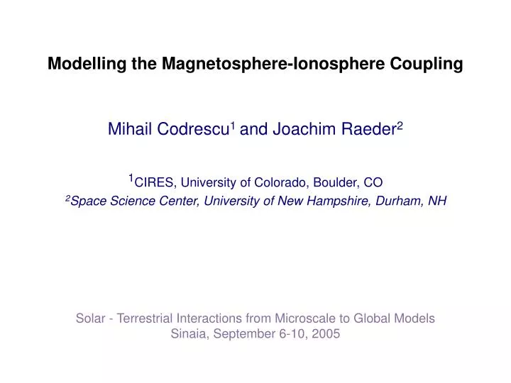
Modelling the Magnetosphere-Ionosphere Coupling Mihail Codrescu 1 and Joachim Raeder 2 1 CIRES, University of Colorado, Boulder, CO 2 Space Science Center, University of New Hampshire, Durham, NH Solar - Terrestrial Interactions from Microscale to Global Models Sinaia, September 6-10, 2005.

E N D
Modelling the Magnetosphere-Ionosphere Coupling Mihail Codrescu1 and Joachim Raeder2 1CIRES, University of Colorado, Boulder, CO 2Space Science Center, University of New Hampshire, Durham, NH Solar - Terrestrial Interactions from Microscale to Global Models Sinaia, September 6-10, 2005
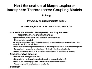
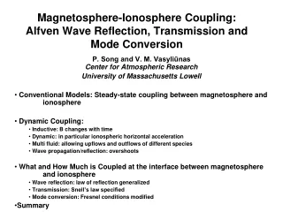
Global modeling of the geospace environment began about 20 years ago with the first simple magnetohydrodynamic (MHD) models of the solar wind - magnetosphere interaction. It is thus a relatively young discipline compared to, for example, the modeling of the atmosphere. However, over this comparatively short period enormous progress has been made. Recently the inclusion of electrodynamic ionosphere models that provide the closure of field-aligned currents (FACs) and the connection between magnetospheric and ionospheric convection has been achieved. The coupling to the ionosphere followed the realization that the ionosphere might, at least in part, control magnetospheric convection, and thus the magnetospheric dynamics in general. In this paper we'll discuss the status of magnetosphere-ionosphere coupling with examples of ionosphere coupling to the inner magnetosphere as described by the Rice Convection Model and to a full magnetosphere MHD code, the OpenGGCM.
Outline Current Systems in the Magnetosphere The Thermosphere Ionosphere System CTIPe and Rice Convection Model coupling MI Coupling MHD Magnetosphere + Rice Convection Model
Current Systems in the Magnetosphere • Magnetopause current at equator and above polar cusp • Region 1 field-aligned current • Region 2 field-aligned current • The symmetric ring current • The partial ring current • The plasma sheet current • The substorm current wedge • Currents NOT SHOWN: • Closure of plasma sheet current • Currents in the polar cusp • Closure of boundary layer current McPherron, R.L., Physical Processes Producing Magnetospheric Substorms and Magnetic Storms, in Geomagnetism, edited by J. Jacobs, pp. 593-739, Academic Press, London, 1991.
The Currents Produced by M-I Coupling • On the dawn side Region 1 current flows downward from the inner edge of the low latitude boundary region • R1 current splits with some flowing over the polar cap and the rest equatorward • At the shielding layer current flows upward as Region 2 current • This current flows westward in the equatorial plane through gradient and curvature drift • On the dusk side the current flows downward as R1 current • It then flows poleward meeting current flowing over the polar cap • The currents combine and flow outward to the inner edge of the dusk boundary layer • Closure from the outer edges of the boundary layers is unknown, but could be through the polar cusp or through the solar wind McPherron, R.L., Physical Processes Producing Magnetospheric Substorms and Magnetic Storms, in Geomagnetism, edited by J. Jacobs, pp. 593-739, Academic Press, London, 1991.
January 9 -10, 1997 T. Matsuo Private Communication, 2004
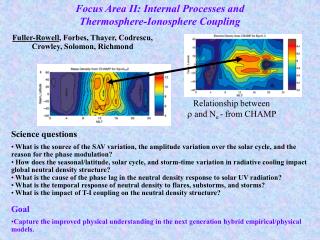
Large Variability Fejer and Scherliess, 2001
What is the source of the vertical drifts? Two Processes: -Prompt Penetration [e.g., Jaggi and Wolf, 1973] -Disturbance dynamo [e.g., Blanc and Richmond, 1980] [Scherliess and Fejer, 1997] Coupled Thermosphere Ionosphere Plasmasphere Electrodynamics (CTIPe) model is used. Maruyama, private communication, 2005
RCM - CTIPe Coupling Experiment • RCM Input: • --polar cap potential drop • --Tsyganenko 2003 storm magnetic field • --plasma sheet density and temperature on the high-latitude boundary RCM run Penetration Electric fields CTIPe Input 5UT 50 -50 5UT Maruyama, private communication, 2005 [Sazykin et al., 2004]
LON=127 Response of Vertical ExB Drift 4 CTIPe Runs: Day Night -----: Quiet time ___: Disturbance Dynamo only (Weimer) ___: Penetration only (RCM) ___: both Disturbance Dynamo (Weimer) & Penetration (RCM) 03/31/01 0UT 24UT LON=289 Night -- Very Dynamic! -- Very Complicated! -- Hard to distinguish the effects! Day (Maruyama, 2005)
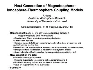
MI Coupling MHD model provides FAC, e- precipitation.Potential solver uses FAC, conductances to compute 2d ionosphere potentialCTIM receives potential, e- precipitation, provides conductances and dynamo currents
OpenGGCM Structure • Sunward of bow shock to distant tail • +-40 RE in Y/Z • R = 3 RE inner boundary with coupling to CTIM (Coupled Thermosphere Ionosphere Model) • Driven by SW B,V,N,T, and F10.7 • Model is available for community use at CCMC: http://ccmc.gsfc.nasa.gov
Typical Numerical Grid Variable, static grid spacing.Can be as small as 100 km near magnetopause, but for storm simulations usually 0.2-0.3 RE at subsolar MP, larger elsewhere.Parallelized using domain decomposition, 4 - 800 processors, various architectures.
Computation Finite difference solution.2. order explicit time integration.2./4. order, flux-limited spatial differences.Yee grid / constrained transport algorithm guarantees div(B)=0.For space weather speed is of essence: ~ real time with 4M cells on ~60 Opteron CPUs.I/O can be a bottleneck.Model provides 3d magnetosphere B, V, N, T; ionosphere FAC, Pot, e- prec, Sig_P, Sig_H, J,…; CTIM provides 3d Vp, Ti, Ne, Nmf2, H+/O+ Tn, N, O/N, ….;
Storms in different shapes and sizes Bastille Day storm stands out among 1998-2001 storms.IMF Bz as large as -60 nT, IEF Ey as large as 70 mV/mDst ~ -300 nT
Bastille Day storm: Geomagnetic activity IMF Bz driverPolar Cap potential.Black: AMIE (G. Lu, NCAR/HAO), green: model.A indices from 60+ stations, model results in red.
Reality check: GOES magnetopause crossings Blue: typical quiet day at GOES.Red: GOES data.Black: model
Polar Cap Potential saturation Predicted versus observed PCP.Empirical models severely overpredict PCP.OpenGGCM is close but on the high side versus AMIE.
Polar Cap Potential saturation IEF Ey is main driver for empirical models.During Bastille Day storm PCP is so saturated there is virtually no Ey dependence.
Saturation mechanism Shortened X-line due to MP erosion explains much of the effect.Equivalent to Siscoe-Hill model: limited R1 system.
Scaled empirical models Empirical models scaled by X-line size fit much better, but still high CPCP.Simple linear model (green) is not adequate.
Limits of predictability • With strong SW forcing tail PS is turbulent. • How can turbulence be characterized? • Is the turbulence in the model the “right” turbulence?
The future: RC and RB coupling • One of the biggest model deficiencies is the lack of proper “inner magnetosphere” physics. • Coupling with RC/RB models is in the works (RCM, Jordanova, Fok models). • Coupling must be both to the magnetosphere (pressure feedback) and ionosphere (e- precipitation, R2 currents). • Replacing CTIM with CTIPe may also be helpful (plasmasphere).
Energy Deposition Viereck, Private communication, 2004
Magnetosphere - Ionosphere Coupling MHD Model Jll, np,Tp E Magnetosphere - Ionosphere Coupler Particle precipitation: Fe, E0 (SH+SP)=Jll Conductivities:Sp, Sh Electric potential: F T/I Model One Way Coupling Two Way Coupling Adapted from Solomon 2004 (www.bu.edu/cism/AG/ppt/SolomonV2.ppt)
MHD magnetosphere model Model region [-400,20]x[-50,50]x[-50,50] RE box Solve MHD equations Anomalous resistivity Numerics: explicit finite difference Outer boundary conditions: solar wind upstream, open ol all other sides Inner boundary conditions: E, v from ionosphre Computing: Parallelized using message passing interface (MPI) 8-64 nodes, but scales well up to 256 nodes