Download
1 / 9
90 likes | 204 Views
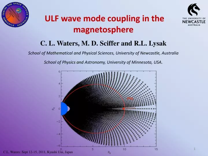
ULF wave mode coupling in the magnetosphere C. L. Waters, M. D. Sciffer and R.L. Lysak School of Mathematical and Physical Sciences, University of Newcastle, Australia School of Physics and Astronomy, University of Minnesota, USA. C.L. Waters: Sept 12-15, 2011, Kyushi Uni, Japan.

E N D
ULF wave mode coupling in the magnetosphere C. L. Waters, M. D. Sciffer and R.L. Lysak School of Mathematical and Physical Sciences, University of Newcastle, Australia School of Physics and Astronomy, University of Minnesota, USA. C.L. Waters: Sept 12-15, 2011, Kyushi Uni, Japan
Electromagnetism and Fluids: MHD Mass continuity Momentum equation For 1-D, B0(x) az Ohm’s Law - from momentum Faraday and Ampere Laws Waters et al., JGR, 2000 C.L. Waters: Sept 12-15, 2011, Kyushi Uni, Japan
VA and FLR with RE Fast mode turning point Waters et al., JGR, 2000 C.L. Waters: Sept 12-15, 2011, Kyushi Uni, Japan
Resonance point : turning point b amplitude polarisation change Phase: VA and FLR C.L. Waters: Sept 12-15, 2011, Kyushi Uni, Japan
2,3-D Coordinate Systems Dipole coordinates are used by many ULF wave models Ok for the magnetosphere Ionosphere is more spherical - inner boundary conditions Lysak 2004 introduced a tilt dipole coordinate system Facilitates ionosphere boundary equations Dipole Coordinates Tilt Dipole Coordinates C.L. Waters: Sept 12-15, 2011, Kyushi Uni, Japan
B3 Contravariant B3 is Normal to the ionosphere current Sheet Current Sheet (constant u3 surface) r = RI Magnetic field r = Re E1 andE2 Covariant E’s lie in the ionosphere current sheet Ground Perfect Conductor Neutral Atmosphere J = X B= 2 Ψ = 0 for B = Ψ Ionosphere Boundary E1 E2 and B3 are continuous across the ionosphere current sheet. The jump in the covariant components of B is directly proportional to the current: Σis the height integrated conductivity tensor, including Pedersen and Hall terms r is the unit normal to the current sheet ∆B is the jump in the covariant (tangential) magnetic field across the current sheet . C.L. Waters: Sept 12-15, 2011, Kyushi Uni, Japan
2½ D ULF Wave Model J is the Jacobian for the coordinate system, m is the azimuth wave number V2 = 1/μ0 ┴ where ┴ = 0(1+c2/ Va2) To evolve the contravariant (superscripts) components into new covariant (subscripts) for the next time step we use: E1 = g11 E1E2 = g22 E2 B1 = g11B1 + g13B3 B2 = g22B2 B3 = g31B1 + g33B3 where gij are the components of the metric tensor given by gij = ei . ej where el are the corresponding covariant basis vectors (see Lysak, JGR, 2004 : Waters and Sciffer, JGR, 2008) C.L. Waters: Sept 12-15, 2011, Kyushi Uni, Japan
The Alfven speed IMAGE, RPI data IRI MSIS FLRs satellite data C.L. Waters: Sept 12-15, 2011, Kyushi Uni, Japan