Download
1 / 83

E N D
Fluid measurements include the determination of pressure, velocity, discharge shock waves, density gradients, turbulence, and viscosity. There are many ways these measurements may be taken, e.g., direct, indirect, gravimetric, volumetric electronic, electromagnetic, and optical. • Direct measurements for discharge consist in the determination of the volume or weight of fluid that passes a section in a given time interval. Indirect methods of discharge measurement require the determination of head, difference in pressure, or velocity at several points in a cross section and, with these, computing the discharge. • The most precise methods are the gravimetric or volumetric determinations, in which the weight or volume is measured by weigh scales or by a calibrated tank for a time interval that is measured by a stopwatch.
9.1 PRESSURE MEASUREMENT • The measurement of pressure is required in many devices that determine the velocity of a fluid stream or its rate of flow, because of the relation between velocity and pressure given by the energy equation. The static pressure of a fluid in motion is its pressure when the velocity is undisturbed by the measurement. • Figure 9.1a indicates one method of measuring static pressure, the piezometer opening. When the flow is parallel, as indicated, the pressure variation is hydrostatic normal to the streamlines; hence, by measuring the pressure at the wall, the pressure at any other point in the cross section can be determined. • The piezometer opening should be small, with length of opening at least twice the diameter, and should be normal to the surface, with no burrs at its edges, because small eddies would form and distort the measurement.
For rough surfaces, the static tube (Fig. 9.1b) may be used. It consists of a tube that is directed upstream with the end closed. It has radial holes in the cylindrical portion downstream from the nose. • The flow is presumed to be moving by the openings as if it were undisturbed. There are disturbances, however, due to both the nose and the right-angled leg that is normal to the flow. • The static tube should be calibrated, as it may read too high or too low. If it does not read true static pressure, the discrepancy normally varies as the square of the velocity of flow by the tube; i.e.,
Figure 9.1 Static-pressure-measuring devices: (a) piezometer opening, (b) static tube.
Such tubes are relatively insensitive to the Reynolds number and to Mach numbers below unity. Their alignment with the flow is not critical, so that an error of but a few percent is to be expected for a yaw misalignment of 15℃. • The piezometric opening may lead to a bourdon gage, a manometer, a micromanometer, of an electronic transducer. The transducers depend upon very small deformations of a diaphragm due to pressure change to create an electronic signal. • The principle may be that of a strain gage and a Wheatstone bridge circuit, or it may rely on motion in a differential transformer, a capacitance chamber, or the piezoelectric behavior of a crystal under stress.
8.2 VELOCITY MEASUREMENT • Since determining velocity at a number of points in a cross section permits evaluating the discharge, velocity measurement is an important phase of measuring flow. Velocity can be found by measuring the time an identifiable particle takes to move a known distance. This is done whenever it is convenient or necessary. • This technique has been developed to study flow in regions which are so small that the normal flow would be greatly disturbed and perhaps disappear if an instrument were introduced to measure the velocity. • A transparent viewing region must be made available, and by means of a strong light and a powerful microscope the very minute impurities in the fluid can be photographed with a high-speed motion-picture camera. From such motion pictures the velocity of the particles, and therefore the velocity of the fluid in a small region, can be determined.
The pitot tube operates on such a principle and is one of the most accurate methods of measuring velocity. In Fig. 9.2 a glass tube or hypodermic needle with a right-angled bend is used to measure the velocity v in an open channel. • The tube opening is directed upstream so that the fluid flows into the opening until the pressure builds up in the tube sufficiently to withstand the impact of velocity against it. Directly in front of the opening the fluid is at rest. • The streamline through 1 leads to the point 2, called the stagnation point, where the fluid is at rest, and there divides and passes around the tube. The pressure at 2 is known from the liquid column within the tube. Bernoulli's equation, applied between points 1 and 2, produces
The equation reduces (9.2.1) (9.2.2) • Practically, it is very difficult to read the height Δh from a free surface. • The pitot tube measures the stagnation pressure, which is also referred to as the total pressure. • The total pressure is composed of two parts, the static pressure h0 and the dynamic pressure Δh, expressed in length of a column of the flowing fluid (Fig. 9.2). The dynamic pressure is related to velocity head by Eq. (9.2.1).
Figure 9.3a illustrates one arrangement. Bernoulli's equation applied from 1 to 2 is (9.2.3) • The equation for the manometer, in units of length of water, is • Simplifying gives (9.2.4) • Substituting for in Eq. (9.2.3) and solving for v results in (9.2.5) • The pitot tube is also insensitive to flow alignment, and an error of only a few percent occurs if the tube has a yaw misalignment of less than 15℃.
Figure 9.3 Velocity measurement: (a) pitot tube and piezometer opening, (b) pitot-static tube.
The static tube and pitot tube may be combined into one instrument, called a pitot-static tube (Fig. 9.3b). Analyzing this system in a manner similar to that in Fig. 9.3a shows that the same relations hold; Eq. (9.2.5) expresses the velocity, but the uncertainty in the measurement of static pressure requires a corrective coefficient C to be applied: (9.2.6) • A particular form of pitot-static tube with a blunt nose, the Prandtl tube, has been so designed that the disturbances due to nose and leg cancel, leaving C = 1 in the equation. For other pitot-static tubes the constant C must be determined by calibration. • The current meter (Fig. 9.4a) is used to measure the velocity of liquid flow in open channels. The cups are so shaped that the drag varies with orientation, causing a relatively slow rotation.
The number of signals in a given time is a function of the velocity. The meters are calibrated by towing them through liquid at known speeds. For measuring high-velocity flow a current meter with a propeller as rotating element is used, as it offers less resistance to the flow. • Air velocities are measured with cup-type or vane (propeller) anemometers Fig (9.4b) which drive generators indicating air velocity directly or drive counters indicating the number of revolutions. • By so designing the vanes that they have very low inertia, employing precision bearings and optical tachometers which effectively take no power to drive them, anemometers can be made to read very low air velocities. They can be sensitive enough to measure the convection air currents which the human body causes by its heat emission to the atmosphere.
Figure 9.4 Velocity-measuring devices: (a) Price current meter for liquids (W. and L.E. Gurley); (b) air anemometer (Taylor Instrument Co).
Velocity Measurement in Compressible Flow • The pitot-static tube may be used for velocity determinations in compressible flow. • Applying Eq. (7.3.7) to points 1 and 2 of Fig. 9.3b with V2=0 gives • The substitution of cp is from Eq. (7.1.8). Equation (7.1.17) then gives • The static pressure p1 may be obtained from the side openings of the pitot tube, and the stagnation pressure may be obtained from the impact opening leading to a simple manometer; or p2 - p1 may be found from the differential manometer.
Positive-Displacement Meters • One volumetric meter, the positive-displacement meter, has pistons or partitions which are displaced by the flowing fluid and a counting mechanism that records the number of displacements in any convenient unit, such as liters. • A common meter is the disk meter, or wobble meter used on many domestic water-distribution systems. The disk oscillates in a passageway, so that a known volume of fluid moves through the meter for each oscillation. • A stem normal to the disk operates a gear train which, in turn, operates a counter. In good condition, these meters are accurate to within 1 percent. When they are worn, the error may be very large for small flows, such as those caused by a leaky faucet.
The flow of natural gas at low pressure is usually measured by a volumetric meter with a traveling partition. The partition is displaced by gas inflow to one end of the chamber in which it operates, and then, by a change in valving, it is displaced to the opposite end of the chamber. • Oil flow or high-pressure gas flow ina pipeline is frequently measured by a rotary meter in which cups or vanes move about an annular opening and displace a fixed volume of fluid for each revolution. Radial or axial pistons may be so arranged that the volume of a continuous flow through them is determined by rotations of a shaft. • Positive-displacement meters normally have no timing equipment that measures the rate of flow. The rate of steady flow may be determined with a stopwatch to record the time for displacement of a given volume of fluid.
9.3 ORIFICES Orifice in a Reservoir • An orifice may be used for measuring the rate of flow out of a reservoir or through a pipe. An orifice in a reservoir or tank may be in the wall or in the bottom. It is an opening, usually round, through which the fluid flows, as in Fig. 9.5. • The area of the orifice is the area of the opening. The portion of the flow that approaches along the wall cannot make a right-angled turn at the opening and therefore maintains a radial velocity component that reduces the jet area. • The cross section where the con traction is greatest is called the vena contracta. The streamlines are parallel throughout the jet at this section, and the pressure is atmospheric.
The head H on the orifice is measured from the center of the orifice to the free surface. The head is assumed to be held constant. • Bernoulli's equation applied from a point 1 on the free surface to the center of the vena contracta, point 2, with local atmospheric pressure as datum and point 2 as elevation datum, neglecting losses, is written • Inserting the values gives (9.3.1) • The ratio of the actual velocity to the theoretical velocity is called the velocity coefficient; that is, and hence (9.3.2-3)
The ratio of jet area at vena contracta to area orifice is symbolized by another coefficient called the coefficient of contraction: (9.3.4) • The area at the vena contracta is CcA0. The actual discharge is thus (9.3.5) • It is customary to combine the two coefficients into a discharge coefficient Cd, (9.3.6) • from which (9.3.7) • There is no way to compute the losses between points 1 and 2; hence, must be determined experimentally. It varies from 0.95 to 0.99 for the square-edged or rounded orifice.
Trajectory method. • By measuring the position of a point on the trajectory of the free jet downstream from the vena contracta (Fig.9.5) the actual velocity Va can be determined if air resistance is neglected. The x component of velocity does not change; therefore, Vat=x0, in which t is the time for a fluid particle to travel from the vena contracta to point 3. • The time for a particle to drop a distance y0 under the action of gravity when it has no initial velocity in that direction is expressed by y0=gt2/2 . After t is eliminated in the two relations, • With V2t determined by Eq.(9.3.1), the ratio VaVt=Cv is known.
Direct measuring ofVa. With a pitot tube placed at the vena contracta, the actual velocity Va is determined. • Direct measuring of jet diameter. With outside calipers, the diameter of jet at the vena contracta may be approximated. This is not a precise measurement and in general is less satisfactory than the other methods. • Use of momentum equation. When the reservoir is small enough to be suspended on knife-equation, as in Fig. 9.6, it is possible to determine the force F that creates the momentum in the jet. With the momentum equation,
Figure 9.6 Momentum method for determination of Cv and Cc
Losses in orifice Flow • The head loss in flow through an orifice is determined by applying the energy equation with a loss term for the distance between points 1 and 2 (Fig. 9.5), • Substituting the values for this case gives (9.3.8) • in which Eq. (8.3.3) has been used to obtain the losses in terms of H and Cv or V2a and Cv.
Example 9.1 • A 75-mm-diameter orifice under a head of 4.88 m discharges 907.6 kg water in 32.6 s. The trajectory was determined by measuring x0=4.76m for a drop of 1.22 m. Determine Cv, Cc, Cd, the head loss per unit gravity force, and the power loss. Solution • The theoretical velocity V2t is • The actual velocity is determined from the trajectory. The time to drop 1.22 m is
and the velocity is expressed by • Then • The actual discharge Qa is • With Eq. (9.3.7)
Hence, from Eq. (9.3.6), • The head loss, from Eq. (9.3.8), is • The power loss is
The Borda mouthpiece (Fig. 9.7), a short, thin-walled tube about one diameter long that projects into the reservoir (re-entrant), permits application of the momentum equation, which yields, one relation between Cv and Cd. • The velocity along the wall of the tank is almost zero at all points; hence, the pressure distribution is hydrostatic. • The final velocity is V2a; the initial velocity is zero; and Qa is the actual discharge. Then • and • Substituting for Qaand V2a and simplifying lead to
Orifice in a Pipe • The square-edged orifice in a pipe (Fig. 9.8) causes a contraction of the jet downstream from the orifice opening. For incompressible flow Bernoulli’s eq’n applied from section 1 to the jet at its vena contracta, section 2, is • The continuity equation relates V1t and V2t with the contraction coefficient Cc=A2/A0, (9.3.9) • After eliminating V1t, • and by solving for V2t the result is
Multiplying by Cv to obtain the actual velocity at the vena contracta gives • And, finally multiplying by the area of the jet, CcA0, produces the actual discharge Q. (9.3.10) • In which Cd=CvCc. In terms of the gage difference R’, Eq.(9.3.10) becomes (9.3.11) • Because of the difficulty in determining the two coefficients separately, a simplified formula is generally used, (9.3.12)
or its equivalent, (9.3.13) • Values of C are given in Fig. 9.9 for the VDI orifice. • By a procedure explained in the next section, Eq.(9.3.12) can be modified by an expansion factor Y (Fig.9.14) to yield actual mass rate of compressible (isentropic) flow. (9.3.14) • The location of the pressure taps is usually so specified that an orifice can be installed in a conduit and used with sufficient accuracy without performing a calibration at the site.
Unsteady Orifice Flow from Reservoirs • In the orifice situations considered, the liquid surface in the reser-voir has beenassumed to be held constant. • The volume discharged from the orifice in time δt is Qδt, which must just equal the reduction in volume in the reservoir in the same time increment (Fig.9.10.). Equating the two expressions gives • Solving for δt and integrating • After substitution for Q, • For the special case of a tank with constant cross section,
Example 9.2 • A tank has a horizontal cross-sectional area of 2 m2 at the elevation of the orifice, and the area varies linearly with elevation so that it is 1 m2 at a horizontal cress section 3 m above the orifice. For a 100-mm-diameter orifice, Cd=0.65, compute the time, in seconds, to lower the surface from 2.5 to 1 m above the orifice. Solution and
9.4 VENTURI METER, NOZZLE, AND OTHER RATE DEVICES Venturi Meter • The venturi meter is used to measure the rate of flow in a pipe. It is generally a casting (Fig 9.12) consisting of • (1) an upstream section which is the same size as the pipe, has a bronze liner, and contains a piezometer ring for measuring static pressure; • (2) a converging conical section; • (3) a cylindrical throat with a bronze liner containing a piezometer ring; • (4) a gradually diverging conical region leading to a cylindrical section the size of the pipe. • A differential manometer is attached to the two piezometer rings. The amount of discharge in incompressible flow is shown to be a function of the manometer reading.
The pressures at the upstream section and throat are actual pressures, and the velocities from Bernoulli's equation are theoretical velocities. When losses are considered in the energy equation, the velocities are actual velocities. • From Fig. 9.12 (9.4.1) • With the continuity equation V1D12=V2D22, (9.4.2) • Equation (9.4.1) can be solved for V2t, • and (9.4.3)
Introducing the velocity coefficient V2a=CvV2t gives (9.4.4) • After multiplying by A2, the actual discharge Q is determined to be (9.4.5) • In units of length of water • Simplifying gives (9.4.6)
By substituting into Eq.(9.4.5), (9.4.7) • The discharge depends upon the gage difference R‘ regardless of the orientation of the venturi meter; whether it is horizontal, vertical, or inclined, exactly the same equation holds. • Experimental results for venturi meters are given in Fig. 9.13. The coefficient may be slightly greater than unity for venturi meters that are unusually smooth inside. This does not mean that there are no losses ; it results from neglecting the kinetic-energy correction factors α1, α2 in the Bernoulli equation. • The loss is about 10 to 15 percent of the head change between sections 1 and 2.
Venturi Meter for Compressible Flow • The theoretical flow of a compressible fluid through a venturi meter is substantially isentropic and is obtained from Egs.(7.3.2), (7.3.6), and (7.3.7). When multiplied by Cv, the velocity coefficient, it yields for mass flow rate (9.4.8) • Equation (9.4.5), when reduced to horizontal flow and modified by insertion of an expansion factor, can be applied to compressible flow (9.4.9) • Values of Y are plotted in Fig. 9.14 for k=1.40.
Flow Nozzle • The ISA (Instrument Society of America) flow nozzle (originally the VDI flow nozzle) is shown in Fig. 9.15. It has no contraction of the jet other than that of the nozzle opening; therefore, the contraction coefficient is unity. • Equations (9.4.5) and (9.4.7) hold equally well for the flow nozzle. For a horizontal pipe (h = 0), Eq. (9.4.5) may be written (9.4.10) in which (9.4.11) • and Δp=p1-p2. The value coefficient C in Fig. 9.15 is for use in Eq. (9.4.10).
Figure 9.15 ISA (VDI) flow nozzle and discharge coefficients.
Example 9.4 • Determine the flow through a 150-mm-diameter water line that contains a 100 mm-diameter flow nozzle. The mercury-water differential manometer has a gage difference of 2501 mm. water temperature is 15°C. Solution • From the data given, S0=13.6, S1=1.0, R'=0.25 m, A2=π/400=0.00785 m2, ρ = 999.1 kg/m3, μ = 0.00114 Pa·s. Substituting Eq. (9.4.11) into Eq. (9.4.7) gives