Download
1 / 16
160 likes | 420 Views
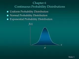
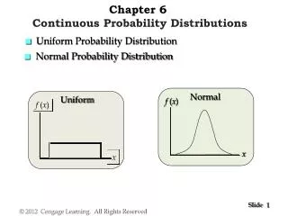
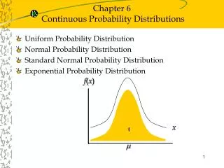
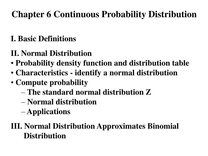
Chapter 6 Continuous Probability Distribution. I. Basic Definitions II. Normal Distribution Probability density function and distribution table Characteristics - identify a normal distribution Compute probability The standard normal distribution Z Normal distribution Applications

E N D
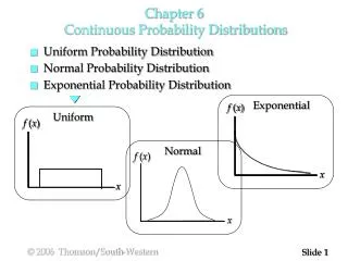
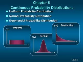
Chapter 6 Continuous Probability Distribution • I. Basic Definitions • II. Normal Distribution • Probability density function and distribution table • Characteristics - identify a normal distribution • Compute probability • The standard normal distribution Z • Normal distribution • Applications • III. Normal Distribution Approximates Binomial Distribution
I. Basic Definitions • Continuous random variable: it takes all values over an interval. • For continuous probability distribution • For an individual value of X: P(X=x) = 0 • For an interval of X: 0 P(x1 X x2) 1 • Probability density function f(x) measures probability for a neighborhood of x. • - It’s not P(X=x). • - We use probability density function to compute cumulative probability. • Cumulative probability P(x1 X x2) Vs. probability function f(x): Area and height. In general,
II. Normal Distribution • Probability density function and distribution table • Probability density function • Probability distribution table: for the • standard normal distribution Z - Table 1 (A-4) • Identify a normal distribution - characteristics • Symmetric and bell-shaped (p.239 Figure 6.3) • Follow the empirical rule (p.241 Figure 6.4) • The total area under the probability curve is 1: • P(- X +) = 1 (p.240) • Two parameters ( and ) determine the distribution: X N(, ) (pp.239-240)
Compute Probability (Outlines) • 1. The standard normal distribution Z N(0, 1) • What are in Table 1? • Value of Z and P(0 Z z) • What can we find by using Z-Table? • - Given an interval of Z, find probability. • - Given probability for an interval of Z, find the interval. • 2. Normal distribution X N(, ) • Can we use Z-Table? • What kind of problems? • - Given an interval of X, find probability. • - Given probability for an interval of X, find the interval.
0 .44 0 -.23 • 1. The standard normal distribution Z N(0, 1) • Given an interval of Z, find probability • Example. P.248 #12 a. P(0 Z .83) = ? P(Z .83) -.5 = .7967 - .5 (Z-Table) = .2967 b. P(-1.57 Z 0) = ? (symmetrical) .5 - P(Z -1.57) = .5 - .0582 (Z-Table) = .4418 c. P(Z > .44) = ? 1 - P(Z ≤ .44) = 1 - .67 (Z-Table) = .33 d. P (Z -.23) = ? 1 - P (Z ≤ -.23) = 1 - .4090 (Z-Table) = .591
0 0 -.71 -1.98 0 .49 Example. P.248 #12 e. P(Z < 1.20) = ? P(Z < 1.20) =.8849 (Z-Table) f. P(Z -.71) = ? P(Z -.71) =.2389 (Z-Table) Example. P.241 #13 a. P(-1.98 Z .49) = ? P(Z .49) – P(Z -1.98)= .6879 + .0239 (Z-Table) = .6640 Homework: p.248 #13 1.20
z .2119 P=? 0 z 1. The standard normal distribution Z N(0, 1) (2) Given probability for an interval of Z, find the interval Example. P.249 #15 Find value of z. a. The area to the left of z is .2119. P(Z z) = .2119 Key: which side is z? Suppose the first picture is correct, the probability is greater than .5 (impossible to be .2119). The second one is correct. z = -.80 (Z-Table) Homework: p.249 #15 0
2. Normal distribution X N(, ) To use Table 1: (1) Given an interval of X, find probability Procedure: X Z Z-Table: P(Z) P(X) = P(Z) Example 1: According to a survey, subscribers to The Wall Street Journal Interactive Edition spend an average of 27 hours per week using the computer at work. Assume the normal distribution applies and that the standard deviation is 8 hours. a. What is the probability a randomly selected subscriber spends less than 11 hours using the computer at work?
Example 1: (continued) b. What percentage of the subscribers spends more than 40 hours per week using the computer at work? c. A person is classified as a heavy user if he or she is in the upper 20% in terms of hours of usage. How many hours must a subscriber use the computer in order to be classified as a heavy user? Solution: X: the number of hours per week using computer at work. X N(, ): = 27, = 8 “a” and “b”: x P; “c”: P x.
P=? 27 11 0.2734 P=? 0 -2 P=? 27 40 0.4484 P=? 0 1.625 • a. P(X < 11) • Z-score for X = 11: • z = (x- )/ = (11 - 27)/8 • = -2 • P(Z < -2) = 0.0228 (Z-Table) • P(X < 11) = P(Z < -2) = .0228 • b. P(X > 40) • Z-score for X = 40: • z = (x- )/ = (40 - 27)/8 • = 1.625 • P(Z > 1.625) = 1 – P(Z < 1.625) • 1 - .9484 = 0.0516 = 5.16%
Example. p.250 #23 • The time needed to complete a final examination in a particular college course is normally distributed with a mean of 80 minutes and a standard deviation of 10 minutes. • What is the probability of completing the exam in one hour or less? • What is the probability that a student will complete the exam in more than 60 minutes but less than 75 minutes? • Assume that the class has 60 students and that the examination period is 90 minutes in length. How many students do you expect will be unable to complete the exam in the allotted time?
P=? 0 -2 P=? 80 60 • Solution: • X: the number of minutes to complete the exam. • X N(, ): = 80, = 10 • “a”, “b” and “c”: x P. • “c”: x P (% of students) the number of students: (60)(% of students) • a. P(X < 60) • Z-score for X = 60: • z = (x- )/ = (60 - 80)/10 • = -2 • P(Z < -2) = 0.0228 • P(X < 60) = P(Z < -2) = .0228 0.2734
P=? 60 75 80 P=? -2 -0.5 80 • b. P(60 < X < 75) • Z-score for X = 60: • z1 = (x- )/ = (60 - 80)/10 • = -2 • Z-score for X = 75: • z2 = (x- )/ = (75 - 80)/10 • = -0.5 • P(-2 < Z < -.5) = P(Z < -.5) – P(Z < -2) • = .3085 - .0228 = .2857 • P(60 < X < 75) = P(-2 < Z < -.5)= .2857
0.3413 P=? 0 1 P=? 80 90 • c. P(X > 90) • Z-score for X = 90: • z = (x- )/ = (90 - 80)/10 • = 1 • P(Z > 1) = 1 – P(Z < 1) • = 1 - .8413 = .1587 • P(X > 90) = P(Z > 1)= .1587 • The number of students = (60)(.1587) = 9.522.
2. Normal distribution X N(, ) To use Table 1: (2) Given probability for an interval of X, find the interval Procedure: X Z Table 1: P(Z) Z x=x+zx Example 1: (Continued) c. A person is classified as a heavy user if he or she is in the upper 20% in terms of hours of usage. How many hours must a subscriber use the computer in order to be classified as a heavy user? Solution: X: the number of hours per week using computer at work. X N(, ): = 27, = 8 . “c”: P x.
0.20 0.20 z=? 27 Solution: • c. P(X > x) = 20%, x=? • X Z: • Key: Which side is x? • The z and x are on the same side. • P(Z < z) = 1- P(Z > z) = 1 - .20 = 0.8 • z ≈ 0.84 (P(Z < z) =.7995 closest to .8) • z x: • x=x+zx • x = 27 + (.84)(8) = 33.72 • Homework: p.250 #23 x=? 0.30 0