Download
1 / 33
330 likes | 534 Views
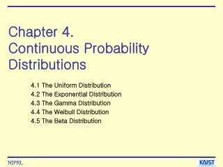
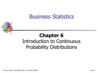
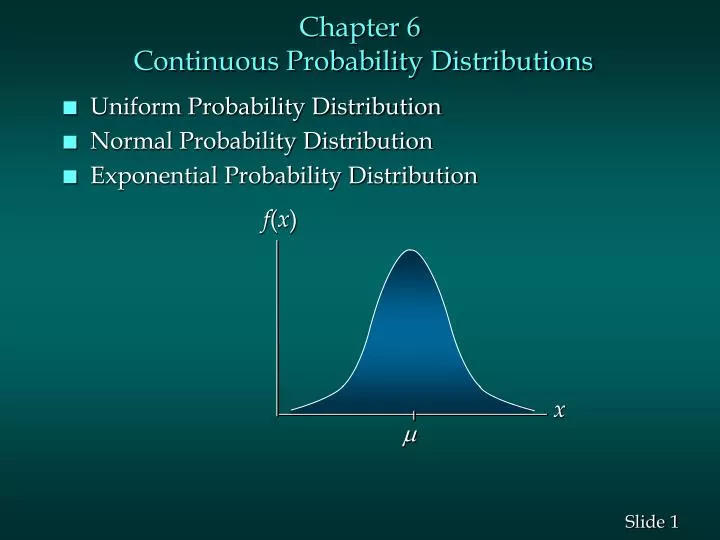
Chapter 6 Continuous Probability Distributions. Uniform Probability Distribution Normal Probability Distribution Exponential Probability Distribution. f ( x ). x. . Continuous Probability Distributions.

E N D
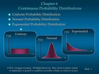
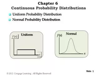
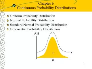
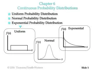
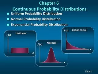
Chapter 6 Continuous Probability Distributions • Uniform Probability Distribution • Normal Probability Distribution • Exponential Probability Distribution f(x) x
Continuous Probability Distributions • A continuous random variable can assume any value in an interval on the real line or in a collection of intervals. • It is not possible to talk about the probability of the random variable assuming a particular value. • Instead, we talk about the probability of the random variable assuming a value within a given interval. • The probability of the random variable assuming a value within some given interval from x1 to x2 is defined to be the area under the graph of the probability density function(概率密度函数)between x1and x2.
Uniform Probability Distribution (均匀概率分布) • A random variable is uniformly distributed whenever the probability is proportional to the interval’s length. • Uniform Probability Density Function f(x) = 1/(b - a) for a<x<b = 0 elsewhere where: a = smallest value the variable can assume b = largest value the variable can assume
Uniform Probability Distribution • Expected Value of x E(x) = (a + b)/2 • Variance of x Var(x) = (b - a)2/12 where: a = smallest value the variable can assume b = largest value the variable can assume
Example: Slater's Buffet • Uniform Probability Distribution Slater customers are charged for the amount of salad they take. Sampling suggests that the amount of salad taken is uniformly distributed between 5 ounces and 15 ounces. The probability density function is f(x) = 1/10 for 5 <x< 15 = 0 elsewhere where: x = salad plate filling weight
Example: Slater's Buffet • Uniform Probability Distribution What is the probability that a customer will take between 12 and 15 ounces of salad? f(x) P(12 <x< 15) = 1/10(3) = .3 1/10 x 5 10 12 15 Salad Weight (oz.)
Example: Slater's Buffet • Expected Value of x E(x) = (a + b)/2 = (5 + 15)/2 = 10 • Variance of x Var(x) = (b - a)2/12 = (15 – 5)2/12 = 8.33
Normal Probability Distribution(正态概率分布) • Graph of the Normal Probability Density Function f(x) x
Normal Probability Distribution • Characteristics of the Normal Probability Distribution • The shape of the normal curve is often illustrated as a bell-shaped curve. • Two parameters, m (mean) and s (standard deviation), determine the location and shape of the distribution. • The highest point on the normal curve is at the mean, which is also the median and mode. • The mean can be any numerical value: negative, zero, or positive. … continued
Normal Probability Distribution • Characteristics of the Normal Probability Distribution • The normal curve is symmetric. • The standard deviation determines the width of the curve: larger values result in wider, flatter curves. • The total area under the curve is 1 (.5 to the left of the mean and .5 to the right). • Probabilities for the normal random variable are given by areas under the curve.
Normal Probability Distribution • % of Values in Some Commonly Used Intervals • 68.26% of values of a normal random variable are within +/- 1standard deviation of its mean. • 95.44% of values of a normal random variable are within +/- 2standard deviations of its mean. • 99.72% of values of a normal random variable are within +/- 3standard deviations of its mean.
Normal Probability Distribution • Normal Probability Density Function where: = mean = standard deviation = 3.14159 e = 2.71828
Standard Normal Probability Distribution • A random variable that has a normal distribution with a mean of zero and a standard deviation of one is said to have a standard normal probability distribution. • The letter z is commonly used to designate this normal random variable. • Converting to the Standard Normal Distribution • We can think of z as a measure of the number of standard deviations x is from .
Example: Grear轮胎公司问题 • Standard Normal Probability Distribution Grear公司刚刚开发了一种新的轮胎,并通过一家全国连锁的折扣商店出售。因为该轮胎是一种新产品,Grear公司的经理们认为是否保证 一定的行驶里程数将是该产品能否被顾客接受的重要因素。在制定这种轮胎的里程质保政策之前,经理们需要知道轮胎行驶里程数的概率信息。 根据对这种轮胎的实际路面测试,公司的工程师小组估计它们的平均行驶里程为36500英里,里程数的标准差为5000。另外,收集到的数据显示,行驶里程数符合正态分布应该是一个合理的假设。 问题是有多大百分比的轮胎能够行驶超过40000英里?换句话说,轮胎行驶里程大于40000英里的概率是多少?
Example: Grear轮胎公司问题 P(x>=40000)=0.5-0.258=0.242 说明:大约有24.2%的轮胎行使里程会超过40000。
Example: Grear轮胎公司问题 • 现在我们假设公司正在考虑一项质量保政策,如果初始购买的轮胎没有能够使用到保证的里程数,公司将以折扣价格为客户更换轮胎。如果公司希望符合折扣条件的轮胎不超过10%,则保证的里程应为多少?
Example: Grear轮胎公司问题 • 分析1:处在均值和未知保证里程数之间的面积必须为40%。
Example: Grear轮胎公司问题 • 分析2:在表中查找0.4,看到该面积大约在均值与小于均值1.28个标准差处之间,即z=-1.28是对应于公司在正态分布中保证里程数的标准正态分布。
Example: Grear轮胎公司问题 • 为了得到对应于z=-1.28的里程数x,我们有: • 因此,30100英时的质量保证将满足只有大约10%的轮胎需要折价更换的要求。也许,根据这一信息,公司将把它的轮胎里程保证设在30000英里。
Exponential Probability Distribution指数概率分布 • Exponential Probability Density Function for x> 0, > 0 where: = mean e = 2.71828
Exponential Probability Distribution(指数概率分布) • Cumulative Exponential Distribution Function where: x0 = some specific value of x
Example: Al’s Carwash • Exponential Probability Distribution The time between arrivals of cars at Al’s Carwash follows an exponential probability distribution with a mean time between arrivals of 3 minutes. Al would like to know the probability that the time between two successive arrivals will be 2 minutes or less. P(x< 2) = 1 - 2.71828-2/3 = 1 - .5134 = .4866
Example: Al’s Carwash • Graph of the Probability Density Function f(x) .4 P(x< 2) = area = .4866 .3 .2 .1 x 1 2 3 4 5 6 7 8 9 10 Time Between Successive Arrivals (mins.)
Relationship between the Poissonand Exponential Distributions (If) the Poisson distribution provides an appropriate description of the number of occurrences per interval (If) the exponential distribution provides an appropriate description of the length of the interval between occurrences