Download
1 / 34
430 likes | 1.01k Views
PROBABILITY AND STATISTICS FOR SCIENTISTS AND ENGINEERS. Special Continuous Probability Distributions Normal Distribution. f(x). x. Normal Distribution – Probability Density Function.

E N D
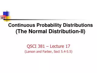
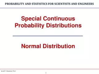
PROBABILITY AND STATISTICS FOR SCIENTISTS AND ENGINEERS Special Continuous Probability DistributionsNormal Distribution
f(x) x Normal Distribution – Probability Density Function A random variable X is said to have a normal (or Gaussian) distribution with parameters and , where - < < and > 0, with probability density function for - < x<
Normal Distribution – Probability Distribution Function • Note: F(x) can not be integrated into a closed form solution.
Standard Normal Distribution If X~ N(, ) and if then Z ~ N(0, 1). A normal distribution with = 0 and = 1, is called the standard normal distribution.
Normal Distribution = f(X) f(z) x z 0
Standard Normal Distribution Table of Probabilities For Z from -8 to 8 http://lyle.smu.edu/~jerrells/courses/newCourses/resource_center/rescen.html (Normal Distribution -> Table -8 to +8)
Normal Distribution - Example The following example illustrates every possible case of application of the normal distribution. Let X~ N(100, 10) Find: (a) P(X < 105.3) (b) P(X 91.7) (c) P(87.1 < X 115.7) (d) the value of x for which P(X x) = 0.05
Normal Distribution – Example Solution (a) Find P(X < 105.3) = P(Z< 0.53) = F(0.53) = 0.7019 f(x) f(z) 0 x 105.3 z 100 0.53 105.3-100 10
Normal Distribution – Example Solution (Continued) (b) Find P(X 91.7) = P(Z ≥-0.83) = 1 – P(Z< -0.83) = 1- F(-0.83) = 1 - 0.2033 = 0.7967 f(x) f(z) z x 0 100 91.7 -0.83 91.7-100 10
Normal Distribution – Example Solution (Continued) (c) Find P(87.1 < X 115.7) f(x) f(x) z x 87.1 100 115.7 -1.29 0 1.57 115.7-100 10 87.1-100 10
Normal Distribution – Example Solution (Continued) (c) P(87.1 < X 115.7)= F(115.7) - F(87.1) = = P(-1.29 < Z < 1.57) = F(1.57) - F(-1.29) = 0.9418 - 0.0985 = 0.8433
Normal Distribution – Example Solution (Continued) (d) Find the value of x for which P(X x) = 0.05 f(x) f(z) 0.05 0.05 z x 1.64 116.4 0 100
Normal Distribution – Example Solution (Continued) (d) if P( X x) = 0.05 P( Z z) = 0.05 then z = 1.64, and P( X x) = therefore , and x - 100 = 16.4 so that x = 116.4
Normal Distribution – Example The time it takes a driver to react to the brake lights on a decelerating vehicle is critical in helping to avoid rear-end collisions. The article ‘Fast-Rise Brake Lamp as a Collision-Prevention Device’ suggests that reaction time for an in-traffic response to a brake signal from standard brake lights can be modeled with a normal distribution having mean value 1.25 sec and standard deviation 0.46 sec. What is the probability that reaction time is between 1.00 and 1.75 seconds? If we view 2 seconds as a critically long reaction time, what is the probability that actual reaction time will exceed this value?
Normal Distribution – Example Solution Find P(1.00 X1.75) f(x) f(z) z x 1.09 -0.54 1.00 1.75 1.25 0 1.75-1.25 0.46 1 -1.25 0.46
Normal Distribution – Example Solution Continued Find P(X >2)
Defective PPM vs Specification Shifted 1.5 σ µ
Application - Tolerance Analysis Convention Normal Probability Distribution 0.00135 0.9973 0.00135 Nominal LTL UTL -3 +3
Statistical Tolerancing - Concept x LTL Nominal UTL
Caution For a normal distribution, the natural tolerance limits include 99.73% of the variable, or put another way, only 0.27% of the process output will fall outside the natural tolerance limits. Two points should be remembered: 1) 0.27% outside the natural tolerances sounds small, but this corresponds to 2700 nonconforming parts per million. 2) If the distribution of process output is non normal, then the percentage of output falling outside 3 may differ considerably from 0.27%.
Normal Distribution - Example The diameter of a metal shaft used in a disk-drive unit is normally distributed with mean 0.2508 inches and standard deviation 0.0005 inches. The specifications on the shaft have been established as 0.2500 0.0015 inches. Determine what fraction of the shafts produced that conform to specifications. Determine the proportion of shafts produced that conform to specificationsif the manufacturing process is re centered, perhaps by adjusting the machine, so that the process mean is equal to the nominal value of 0.2500.
Normal Distribution - Example Solution (a) (b) f(x) 0.2500 nominal x 0.2515 USL 0.2485 LSL 0.2508 f(x) nominal x 0.2485 LSL 0.2515 USL 0.2500
Normal Distribution - Example Solution (a) Thus, we would expect the process yield to be approximately 91.92%; that is, about 91.92% of the shafts produced conform to specifications. Note that almost all of the nonconforming shafts are too large, because the process mean is located very near to the upper specification limit.
Normal Distribution - Example Using a normal probability distribution as a model for a quality characteristic with the specification limits at three standard deviations on either side of the mean. Now it turns out that in this situation the probability of producing a product within these specifications is 0.9973, which corresponds to 2700 parts per million (ppm) defective. This is referred to as three-sigma quality performance, and it actually sounds pretty good. However, suppose we have a product that consists of an assembly of 100 components or parts and all 100 parts must be non-defective for the product to function satisfactorily.
Normal Distribution – Example Solution The probability that any specific unit of product is non-defective is 0.9973 x 0.9973 x . . . x 0.9973 = (0.9973)100 = 0.7631 That is, about 23.7% of the products produced under three sigma quality will be defective. This is not an acceptable situation, because many high technology products are made up of thousands of components. An automobile has about 200,000 components and an airplane has several million!