Download
1 / 38
380 likes | 678 Views
Microarray Basics. Part 2: Data normalization, data filtering, measuring variability. Log transformation of data. Most data bunched in lower left corner Variability increases with intensity. Data are spread more evenly Variability is more even. Simple global normalization

E N D
Microarray Basics Part 2: Data normalization, data filtering, measuring variability
Log transformation of data Most data bunched in lower left corner Variability increases with intensity Data are spread more evenly Variability is more even
Simple global normalization to try to fit the data Slope does not equal 1 means one channel responds more at higher intensity Non zero intercept means one channel is consistently brighter Non straight line means non linearity in intensity responses of two channels
Linear regression of Cy3 against Cy5
MA plots Regressing one channel against the other has the disadvantage of treating the two sets of signals separately Also suggested that the human eye has a harder time seeing deviations from a diagonal line than a horizontal line MA plots get around both these issues Basically a rotation and rescaling of the data A= (log2R + log2G)/2 X axis M= log2R-log2G Y axis
Scatter plot of intensities MA plot of same data
Non linear normalization Normalization that takes into account intensity effects Lowess or loess is the locally weighted polynomial regression User defines the size of bins used to calculate the best fit line Taken from Stekal (2003) Microarray Bioinformatics
Adjusted values for the x axis (average intensity for each feature) calculated using the loess regression Should now see the data centred around 0 and straight across the horizontal axis
Spatial defects over the slide • In some cases, you may notice a spatial bias of the two channels • May be a result of the slide not lying completely flat in the scanner • This will not be corrected by the methods discussed before
Regressions for spatial bias • Carry out normal loess regression but treat each subgrid as an entire array (block by block loess) • Corrects best for artifacts introduced by the pins, as opposed to artifacts of regions of the slide • Because each subgrid has relatively few spots, risk having a subgrid where a substantial proportion of spots are really differentially expressed- you will lose data if you apply a loess regression to that block • May also perform a 3-D loess- plot log ratio for each feature against its x and y coordinates and perform regression
Between array normalization • Previous manipulations help to correct for non-biological differences between channels on one array • In order to compare across arrays, also need to take into account technical variation between slides • Can start by visualizing the overall data as box plots • Looking at the distributions of the log ratios or the log intensities across arrays
Extremes of distribution Std Dev of distribution with mean Extremes of distribution
Data Scaling • Makes mean of • distributions equal • Subtract mean • log ratio • from each log ratio • Mean of measurements • will be zero
Data Centering • Makes means and • standard deviations equal • Do as for scaling, • but also divide by the • mean standard deviation • Will have means intensity • measurements of zero, • standard deviations of 1
Distribution normalization • Makes overall distributions identical between arrays • Centre arrays • For each array, order centered intensities from highest to lowest • Compute new distribution whose lowest value is average of all lowest values, and so on • Replace original data with new values for distribution
Some key points • Design the experiment based on the questions you want to ask • Look at your TIFF images • Look at the raw data with scatter plots and MA plots • Normalize within arrays to remove systematic variability between channels • Scale between arrays prior to comparing results in a data set
Data Filtering (flagging of data) • Can use data filtering to remove or flag features that one might consider to be unreliable • May base the filter on parameters such as individual intensity, average feature intensity, signal to noise ratio, standard deviation across a feature
Using intensity filters • Object is to remove features that have measurements close to background levels- may see large ratios that reflect small changes in very small numbers • May want to set the filter as anything less than 2 times the standard deviation of the background
If using signal to noise ratio, keep in mind that the numbers calculated by QuantArray are: spot intensity/std dev of background Should see that the S/N ratio increase at higher intensity Taken from DNA Microarray Data Analysis (CSC) http://www.csc.fi/oppaat/siru/
Removing outliers • May want to simply remove outliers- some estimates are that the extreme ends of the distribution should be considered outliers and removed (0.3% at either end) • Also want to remove saturated values (in either channel)
Filtering based on replicates • We expect to see A1B2 B1 A2 = 1 * • Consider two replicates with dyes swapped A1 and B2 B1 A2 • We can calculate and eliminate spots with the greatest uncertainty: >2
Replicate Filtering • Plot of the log • ratios of 2 replicates • Remove the data • in red based on • deviation of 2 • st dev Taken from Quakenbush (2002) Nat Genet Supp 32
Z-scores • The uncertainty in measurements increases as intensity decreases • Measurements close to the detection limit are the most uncertain • Can calculate an intensity-dependent Z-score that measures the ratio relative to the standard deviation in the data: Z = log2(R/G)-/
Intensity-dependent Z-score Z > 2 is at the 95.5% confidence level
Small spots with high intensity penalized Large spots may be print defects Signal to noise ratio to define confidence Degree of local background Variation from average background Defined as a threshold, not a continuous function Approaches to using filtering algorithms qsize qsignal to noise qlocal background qbackground variability qsaturated qcom = composite quality score based on the continuous and discrete functions listed above Taken from Wang et al (2001) NAR 29: e75
qcom in relation to log ratio plot Taken from Wang et al (2001) NAR 29: e75
Measuring and Quantifying Variability • Variability may be measured: • Between replicate features on an array • Between two replicates of a sample on an array • Between two replicates of a sample on different arrays • Between different samples in a population
Quantifying variables in microarray data • Measured value for each feature is a combination of the true gene expression, and the sources of variation listed • Each component of variation will have its own distribution with a standard deviation which can be measured
Variability between replicate features • Requires that features are printed multiple times on a chip • Optimal if the features are not printed side by side • Need to calculate this variability separately for the 2 channels
Calculate mean of each replicate Calculate the deviation from the mean for each replicate Produce MA plots 0 If needed, can normalize Diff (Rep1) Calculate std dev of errors Ch1 ave log intensity If the error distribution is ~ normal, you can calculate v Frequency Ch1 Difference
Variability between channels • Perform a self to self hybridization • Perform all the normalization procedures discussed earlier • The variation that is left is going to be due to random variability in measurement between the 2 channels
Variability between arrays • Same samples on different arrays (or just use the common reference sample in a larger experiment) • Now are calculating both the variability due to the manufacturing of different arrays, and the variability of different hybridizations- these are confounded variables
Why calculate these values? • Gives an estimate of comparability in quality between experiments • Gives an estimate of noise in the data relative to population variation • Can be used to track optimization of experiment
Variability between individuals • This is the population variability number that is used in the power calculation • Generally will find that this is the largest source of variation and this is the one that will not be decreased by improving the experimental system
How to calculate population variability • Calculate log ratio of each gene relative to the reference sample • Calculate the average log ratio for each gene across all samples • For each gene in each sample, subtract the log ratio from the average log ratio • Plot the distribution of deviations and calculate the standard deviation (and v)
Part 3-Data Analysis • How to choose the interesting genes in your experiment • How to study relationships between groups of genes identified as interesting • Classification of samples