Download
1 / 13
130 likes | 141 Views
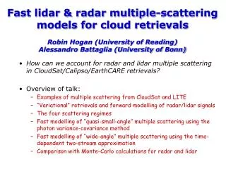
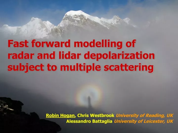
Fast forward modelling of radar and lidar depolarization subject to multiple scattering. Robin Hogan , Chris Westbrook University of Reading, UK Alessandro Battaglia University of Leicester, UK. Examples of multiple scattering. Stratocumulus. Surface echo.

E N D
Fast forward modelling of radar and lidar depolarization subject to multiple scattering Robin Hogan, Chris Westbrook University of Reading, UK Alessandro Battaglia University of Leicester, UK
Examples of multiple scattering Stratocumulus Surface echo Apparent echo from below the surface Intense thunderstorm • LITE lidar (l<r, footprint~1 km) • CloudSat radar (l>r)
Depolarization induced by multiple scattering • Can we model effect of multiple scattering on depolarization? • Potentially very useful information on extinction (e.g. Sassen & Petrilla 1986) Radar: Battaglia et al. (2007) Lidar: Observations at Chilbolton
Overview • Lidar observations in liquid clouds difficult to interpret quantitatively • Difficult to correct for strong attenuation • Radar & lidar multiple scattering contains useful info on extinction • Information mostly in the tail - see Nicola Pounder’s talk on Friday • Depolarization induced by multiple scattering contains more info • Information content first noted by Sassen and Petrilla (1986) • Provides a range-resolved index of multiple scattering • Useful for spaceborne radar: is apparent echo from low in a storm actually from radiation that has just bounced around at cloud top? • Useful for spaceborne lidar: can we retrieve the extinction profile in optically thick liquid clouds? • Challenge: write a fast forward model to use in radar & lidar retrievals • May need to be quite heuristic…
Scattering regimes • Regime 2: Small-angle multiple scattering • Only for wavelength much less than particle size, e.g. lidar & ice clouds • Fast Photon Variance-Covariance (PVC) model of Hogan (2008) • Depolarization due to backscatter slightly away from 180 degrees • Regime 3: Wide-angle multiple scattering • Fast Time Dependent Two Stream (TDTS) method of Hogan & Battaglia • Depolarization increases with number of scattering events • Regime 1: Single scattering • Apparent backscatter b’is easy to calculate • Zero depolarization from droplets Footprint x
A typical Mie phase function for a distribution of droplets Fraction of cross-polar rather than co-polar scattered radiation Forward scattering is unpolarized The glory is polarized
Photon Variance-Covariance methodHogan (JAS 2008): small-angle lidar scattering • Equivalent medium theorem (Katsev et al. 1997): • Use double optical depth on outward journey and zero on return • Apparent backscatter is fraction of photon distribution in FOV • Calculate at each gate: • Total energy P • Position variance • Direction variance • Covariance g • Backscatter co-angle variance • Construct distribution of backscatter co-angles • Convolve with either total, co- or cross-polar phase function • Infrastructure to do this already present in Hogan (2008) model to account for shape of total phase function z s r
Time-dependent 2-stream approximationHogan and Battaglia (JAS 2008): wide-angle scattering Describe diffuse flux in terms of outgoing stream I+ and incoming stream I–, and numerically integrate the following coupled PDEs: I+ and I– are used to calculate total (unpolarized) backscatter btot = b|| + bT Source Scattering from the quasi-direct beam into each of the streams Timederivative Remove this and we have the time-independent two-stream approximation used in weather models Gain by scattering Radiation scattered from the other stream Spatial derivative A bit like an advection term, representing how much radiation is upstream Loss by absorption or scattering Some of lost radiation will enter the other stream
...with depolarization Define “co-polar weighted” streams K+ and K– and use them to calculate the co-polar backscatter bco = b|| – bT: Evolution of these streams governed by the same equations but with a loss term related to the rate at which scattering is taking place, since every scattering event randomizes the polarization and hence reduces the memory of the original polarization: Where is the “fraction of the original polarization that is retained” every scattering event (to be determined by comparison with Monte Carlo calculations provided by Alessandro Battaglia) Depolarization ratio is then calculated from
Interlude for gratuitous animation • Animation of unpolarized scalar flux (I++I–) • Colour scale is logarithmic • Represents 5 orders of magnitude • Domain properties: • 500-m thick • 2-km wide • Optical depth of 20 • No absorption • In this simulation the lateral distribution is Gaussian at each height and each time
Compare with Alessandro Battaglia’s rigorous Monte Carlo model I3RC case 1 isotropic scattering: use single scattering + TDTS model (no forward lobe so no need to treat small-angle scattering) Best fit to depolarization with = 0.75, independent of field of view Evaluation in isotropic conditions
Evaluation in Mie scattering conditions • I3RC case 5: PVC for small-angle and TDTS for wide-angle scattering • Small-angle scattering: excellent fit at close range • Wide-angle scattering: best fit achieved for = 0.6f + 0.85(1–f), where f is the fraction of energy remaining in the field-of-view of the lidar • New model appears to perform well for different fields of view Wide-angle scattering dominates Small-angle scattering dominates
We have developed a fast forward model for the depolarization effects of multiple scattering Applicable to lidar in liquid clouds, yet to be tested for radar Less useful for lidar in ice clouds because of the uncertain single-scattering depolarization Next steps Refine coefficients for different droplet size distributions Incorporate into retrieval scheme (talk on Friday for possible framework) Non-polarized multiple scattering code freely available from http://www.met.rdg.ac.uk/clouds/multiscatter Combines two fast multiple scattering models, PVC & TDTS Includes C & Fortran-90 interfaces, adjoint model, HSRL capability... For lidar, much more accurate than Platt’s approximation with h = 0.7 Can be used in retrievals and in instrument simulators Fast: One profile can cost the same as a single Monte Carlo photon! Outlook