Download
1 / 22
220 likes | 369 Views
The time-dependent two-stream method for lidar and radar multiple scattering Robin Hogan (University of Reading) Alessandro Battaglia (University of Bonn). To account for multiple scattering in CloudSat and CALIPSO retrievals we need a fast forward model to represent this effect Overview:

E N D
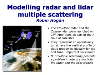
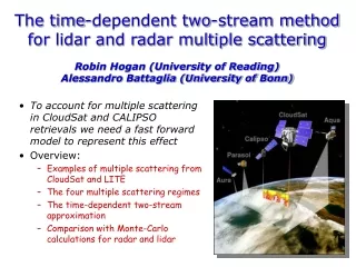
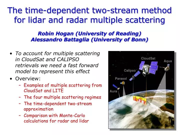
The time-dependent two-stream method for lidar and radar multiple scatteringRobin Hogan (University of Reading)Alessandro Battaglia (University of Bonn) To account for multiple scattering in CloudSat and CALIPSO retrievals we need a fast forward model to represent this effect Overview: Examples of multiple scattering from CloudSat and LITE The four multiple scattering regimes The time-dependent two-stream approximation Comparison with Monte-Carlo calculations for radar and lidar
Examples of multiple scattering Stratocumulus Surface echo Apparent echo from below the surface Intense thunderstorm • LITE lidar (l<r, footprint~1 km) CloudSat radar (l>r)
Scattering regimes • Regime 2: Small-angle multiple scattering • Occurs when Ql~ x • Only for wavelength much less than particle size, e.g. lidar & ice clouds • No pulse stretching • Regime 3: Wide-angle multiple scattering • Occurs when l~ x Mean free path l • Regime 0: No attenuation • Optical depth d<< 1 • Regime 1: Single scattering • Apparent backscatter b’is easy to calculate from d at range r: b’(r) =b(r)exp[-2d(r)] Footprint x
New radar/lidar forward model • CloudSat and CALIPSO record a new profile every 0.1 s • Delanoe and Hogan (JGR 2008) developed a variational radar-lidar retrieval for ice clouds; intention to extend to liquid clouds and precip. • It needs a forward model that runs in much less than 0.01 s • Most widely used existing lidar methods: • Regime 2: Eloranta (1998) – too slow • Regime 3: Monte Carlo – much too slow! • Two fast new methods: • Regime 2: Photon Variance-Covariance (PVC) method (Hogan 2006, Applied Optics) • Regime 3: Time-Dependent Two-Stream (TDTS) method (this talk) • Sum the signal from the relevant methods: • Radar: regime 1 (single scattering) + regime 3 (wide-angle scattering) • Lidar: regime 2 (small-angle) + regime 3 (wide-angle scattering)
Regime 3: Wide-angle multiple scattering Space-time diagram • Make some approximations in modelling the diffuse radiation: • 1-D: represent lateral transport as modified diffusion • 2-stream: represent only two propagation directions I–(t,r) 60° 60° I+(t,r) 60° r
Time-dependent 2-stream approx. • Describe diffuse flux in terms of outgoing stream I+ and incoming stream I–, and numerically integrate the following coupled PDEs: • These can be discretized quite simply in time and space (no implicit methods or matrix inversion required) Source Scattering from the quasi-direct beam into each of the streams Timederivative Remove this and we have the time-independent two-stream approximation Gain by scattering Radiation scattered from the other stream Loss by absorption or scattering Some of lost radiation will enter the other stream Spatial derivative Transport of radiation from upstream Hogan and Battaglia (2008, to appear in J. Atmos. Sci.)
Lateral photon transport • What fraction of photons remain in the receiver field-of-view? • Calculate lateral standard deviation: x y • Diffusion theory predicts superluminal travel when the mean number of scattering events n = ct/ltis small: • In ~1920, Ornstein and Fürth independently solved the Langevin equation to obtain the correct description:
Modelling lateral photon transport • Model the lateral variance of photon position, , using the following equations (where ): • Then assume the lateral photon distribution is Gaussian to predict what fraction of it lies within the field-of-view • Resulting method is O(N2) efficient Additional source Increasing variance with time is described by Ornstein-Fürth formula
Simulation of 3D photon transport • Animation of scalar flux (I++I–) • Colour scale is logarithmic • Represents 5 orders of magnitude • Domain properties: • 500-m thick • 2-km wide • Optical depth of 20 • No absorption • In this simulation the lateral distribution is Gaussian at each height and each time
Monte Carlo comparison: Isotropic • I3RC (Intercomparison of 3D radiation codes) lidar case 1 • Isotropic scattering, semi-infinite cloud, optical depth 20 Monte Carlo calculations from Alessandro Battaglia
Monte Carlo comparison: Mie • I3RC lidar case 5 • Mie phase function, 500-m cloud Monte Carlo calculations from Alessandro Battaglia
Monte Carlo comparison: Radar • Mie phase functions, CloudSat reciever field-of-view Monte Carlo calculations from Alessandro Battaglia
Ongoing work • Apply to “Quickbeam”, the CloudSat simulator (done) • Predict Mie and Rayleigh channels of HSRL lidar (done for PVC) • Implement TDTS in CloudSat/CALIPSO retrieval (PVC already implemented for lidar) • More confidence in lidar retrievals of liquid water clouds • Can interpret CloudSat returns in deep convection • But need to find a fast way to estimate the Jacobian of TDTS • Add the capability to have a partially reflecting surface • Apply to multiple field-of-view lidars • The difference in backscatter for two different fields of view enables the multiple scattering to be interpreted in terms of cloud properties • Predict the polarization of the returned signal • Difficult but useful for both radar and lidar Code available from www.met.rdg.ac.uk/clouds/multiscatter
Monte Carlo comparison: H-G • I3RC lidar case 3 • Henyey-Greenstein phase function, semi-infinite cloud, absorption Monte Carlo calculations from Alessandro Battaglia
How important is multiple scattering for CALIPSO? • Ice clouds: • FOV such that small-angle scattering almost saturates: satisfactory to use Platt’s approximation with h=0.5 • Liquid clouds: • Essential to include wide-angle scattering for optically thick clouds
The basics of a variational retrieval scheme We need a fast forward model that includes the effects of multiple scattering for both radar and lidar Delanoë and Hogan (JGR 2008) New ray of data First guess of profile of cloud/aerosol properties (IWC, LWC, re …) Forward model Predict radar and lidar measurements (Z, b…) andJacobian (dZ/dIWC …) Gauss-Newton iteration step Clever mathematics to produce a better estimate of the state of the atmosphere Compare to the measurements Are they close enough? No Yes Calculate error in retrieval Proceed to next ray
Phase functions • Radar & cloud droplet • l >> D • Rayleigh scattering • g ~ 0 • Radar & rain drop • l~ D • Mie scattering • g ~ 0.5 • Lidar & cloud droplet • l << D • Mie scattering • g ~ 0.85 Asymmetry factor Q q
Regime 2 Equivalent medium theorem: use lidar FOV to determine the fraction of distribution that is detectable (we can neglect the return journey) Calculate at each gate: • Total energy P • Position variance • Direction variance • Covariance z s r • Photon variance-covariance (PVC) method • Photon distribution is estimated considering all orders of scattering with O(N 2) efficiency (Hogan 2006, Appl. Opt.) • O(N ) efficiency is possible but slightly less accurate (work in progress!) • Eloranta’s (1998) method • Estimate photon distribution at range r, considering all possible locations of scattering on the way up to scattering order m • Result is O(N m/m !) efficient for an N -point profile • Should use at least 5th order for spaceborne lidar: too slow Forward scattering events s r
Wide field-of-view: forward scattered photons may be returned Narrow field-of-view: forward scattered photons escape Comparison of Eloranta & PVC methods • For Calipso geometry (90-m field-of-view): • PVC method is as accurate as Eloranta’s method taken to 5th-6th order Ice cloud Molecules Liquid cloud Aerosol Download code from: www.met.rdg.ac.uk/clouds