Download
1 / 25
290 likes | 348 Views
ME 130 Applied Engineering Analysis. Chapter 6 Review of Fourier Series and Its Applications in Mechanical Engineering Analysis Tai-Ran Hsu, Professor Department of Mechanical and Aerospace Engineering San Jose State University San Jose, California, USA. 2017 version. Chapter Outline.

E N D
ME 130 Applied Engineering Analysis Chapter 6 Review of Fourier Series and Its Applications in Mechanical Engineering Analysis Tai-Ran Hsu, Professor Department of Mechanical and Aerospace Engineering San Jose State University San Jose, California, USA 2017 version
Chapter Outline ● Introduction ● Mathematical expressions of Fourier series ● Application in engineering analysis ● Convergence of Fourier series
Introduction Jean Baptiste Joseph Fourier 1749-1829 A French mathematician Major contributions to engineering analysis: ● Mathematical theory of heat conduction (Fourier law of heat conduction in Chapter 3) ● Fourier series representing periodical functions ● Fourier transform Similar to Laplace transform, but for transforming variables in the range of (-∞ and +∞) - a powerful tool in solving differential equations
Periodic Physical Phenomena: Motions of ponies Forces on the needle
Machines with Periodic Physical Phenomena A stamping machine involving cyclic punching of sheet metals In a 4-stroke internal combustion engine: Cyclic gas pressures on cylinders, and forces on connecting rod and crank shaft
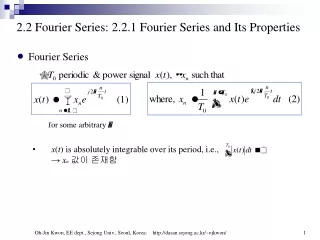
Mathematical expressions for periodical signals from an oscilloscope by Fourier series:
The periodic variation of gas pressure in a 4-stoke internal combustion engine: The P-V Diagram P = gas pressure in cylinders But the stroke l varies with time of the rotating crank shaft, so the time-varying gas pressure is illustrated as: T T So, P(t) is a periodic function with period T Next revolution One revolution
FOURIER SERIES – The mathematical representation of periodic physical phenomena ● Mathematical expression for periodic functions: ● If f(x) is a periodic function with variable x in ONE period 2L ● Then f(x) = f(x±2L) = f(x±4L) = f(x± 6L) = f(x±8L)=……….=f(x±2nL) where n = any integer number Period: ( -π, π) or (0, 2π) Period = 2L: t-4L t-2L t
Mathematical Expressions of Fourier Series ●Required conditions for Fourier series: ● The mathematical expression of the periodic function f(x) in one period must be available ● The function in one period is defined in an interval (c < x < c+2L) in which c = 0 or any arbitrarily chosen value of x, and L = half period ● The function f(x) and its first order derivative f’(x) are either continuous or piece-wise continuous in c < x < c+2L ●The mathematical expression of Fourier series for periodic function f(x) is: (6.1) where ao, an and bn are Fourier coefficients, to be determined by the following integrals: (6.2a) (6.2b)
Example 6.1 Derive a Fourier series for a periodic function with period (-π, π): We realize that the period of this function 2L = π – (-π) = 2π The half period is L = π If we choose c = -π, we will have c+2L = -π + 2π = π Thus, by using Equations (6.1) and (6.2), we will have: and Hence, the Fourier series is: (6.3) with (6.4a) (6.4b) We notice the period (-π, π) might not be practical, but it appears to be common in many applied math textbooks. Here, we treat it as a special case of Fourier series.
Example 6.2 Derive a Fourier series for a periodic function f(x) with a period (-ℓ, ℓ) Let us choose c = -ℓ, and the period 2L = ℓ - (-ℓ) = 2ℓ, and the half period L = ℓ Hence the Fourier series of the periodic function f(x) becomes: (6.5) with (6.6a) (6.6b)
Example 6.3 Derive a Fourier series for a periodic function f(x) with a period (0, 2L). As in the previous examples, we choose c = 0, and half period to be L. We will have the Fourier series in the following form: The corresponding Fourier series thus has the following form: (6.7) (6.8a) (6.8b) (6.8c) Periodic functions with periods (0, 2L) are more realistic. Equations (6.7) and (6.8) are Thus more practical in engineering analysis.
The class is encouraged to study Examples 6.4 and 6.5 Example(Problem 6.4 and Problem (3) of Final exam S09) Derive a function describing the position of the sliding block M in one period in a slide mechanism as illustrated below. If the crank rotates at a constant velocity of 5 rpm. • Illustrate the periodic function in three periods, and • Derive the appropriate Fourier series describing the position of the sliding block x(t) in which t is the time in minutes N
Solution: (a) Illustrate the periodic function in three periods: Determine the angular displacement of the crank: We realize the relationship: rpm N = ω/(2π), and θ = ωt, where ω = angular velocity and θ = angular displacement relating to the position of the sliding block For N = 5 rpm, we have: Based on one revolution (θ=2π) corresponds to 1/5 min. We thus have θ = 10πt ω R θ A B x one revolution Dead-end A: x = 0 t = 0 Dead-end B: x = 2R t = 1/5 min Position of the sliding block along the x-direction can be determined by: x = R – RCosθ x(t) = R – RCos(10πt) = R[1 – Cos(10πt)] 0 < t < 1/5 min or
We have now derived the periodic function describing the instantaneous position of the sliding block as: (a) x(t) = R[1 – Cos(10πt)] 0 < t < 1/5 min ω R θ A B x One revolution Dead-end A: x = 0 t = 0 Dead-end B: x = 2R t = 1/5 min Graphical representation of function in Equation (a) can be produced as: x(t) x(t) = R[1 – Cos(10πt)] 2R R 0 Time, t (min) Θ = 2π π/2 π 3π/2 Time t = 1/10 0 1/5 min One revolution 2nd period 3rd period (one period)
(b) Formulation of Fourier Series: We have the periodic function: x(t) = R[1 – Cos(10πt)] with a period: 0 < t < 1/5 min If we choose c = 0 and period 2L = 1/5, we will have the Fourier series expressed in the following form by using Equations (6.7) and (6.8): (b) with (c) We may obtain coefficient ao from Equation (c) to be ao = 0: The other coefficient bn can be obtained by: (d)
Convergence of Fourier Series We have learned the mathematical representation of periodic functions by Fourier series In Equation (6.1): (6.1) This form requires the summation of “INFINITE” number of terms, which is UNREALISTIC. The question is “HOW MANY” terms one needs to include in the summation in order to reach an accurate representation of the required periodic function [i.e., f(x) in one period]? The following example will give some idea on the relationship of the “number of terms in the Fourier series to represent the periodic function”: Example 6.6 Derive the Fourier series for the following periodic function:
This function can be graphically represented as: We identified the period to be: 2L = π- (-π) = 2π, and from Equation (6.3), we have: (a) with (b) and (c) or For the case n =1, the two coefficients become: and
The Fourier series for the periodic function with the coefficients become: (d) The Fourier series in Equation (b) can be expanded into the following infinite series: (e) Let us now examine what the function would look like by including different number of terms in expression (c): Case 1: Include only one term: Graphically it will look like Observation: Not even closely resemble - The Fourier series with one term does not converge to the function!
Case 2: Include 2 terms in Expression (b): Observation: A Fourier series with 2 terms has shown improvement in representing the function Case 3: Include 3 terms in Expression (b): Observation: A Fourier series with 3 terms represent the function much better than the two previous cases with 1 and 2 terms.
Use four terms in Equation (e): Solid lines = function Dotted lines = Fourier series with 4 terms Conclusion: Fourier series converges better to the periodic function with more terms included in the series. Practical consideration: It is not realistic to include infinite number of terms in the Fourier series for complete convergence. Normally an approach with 20 terms would be sufficiently accurate in representing most periodic functions
Convergence of Fourier Series at Discontinuities of Periodic Functions Fourier series in Equations (6.1) to (6.3) converges to periodic functions everywhere except at discontinuities of piece-wise continuous function such as: = f1(x) 0 < x < x1 = f2(x) x1 < x <x2 = f3(x) x2 < x < x4 f(x) = < The periodic function f(x) has discontinuities at: xo, x1 , x2 and x4 The Fourier series for this piece-wise continuous periodic function will NEVER converge at these discontinuous points even with ∞ number of terms ●The Fourier series in Equations (6.1), (6.2) and (6.3) will converge every where to the function except these discontinuities, at which the series will converge HALF-WAY of the function values at these discontinuities.
Convergence of Fourier Series at Discontinuities of Periodic Functions Convergence of Fourier series at HALF-WAY points: at Point (1) at Point (2) at Point (3) same value as Point (1)
Example 6.8: convergence of Fourier series of piece-wise continuous function in one period: The periodic function in one period: The function has a period of 4 but is discontinuous at: t = 1 and t = 4 Derive the Fourier series to be: with: and Draw the curves represented by the above Fourier series with different number of terms to illustrate the convergence of the series:
With fifteen terms (n = 15): With three terms (n = 3): Converges well with 80 terms!! Observe the convergence of Fourier series at DISCONTINUITIES With eighty terms (n = 80):