Download

1 / 45
460 likes | 690 Views
Fourier Series (Spectral) Analysis. Fourier Series Analysis. Suitable for modelling seasonality and/or cyclicalness Identifying peaks and troughs. A sine wave is a repeating pattern that goes through one cycle every 2 (i.e. 2 3.141593 = 6.283186) units of time. For example,.

E N D
Fourier Series Analysis • Suitable for modelling seasonality and/or cyclicalness • Identifying peaks and troughs
A sine wave is a repeating pattern that goes through one cycle every 2 (i.e. 2 3.141593 = 6.283186) units of time. • For example,
Since Wave Phase Shifts Y = sin (x) Z = sin (x + 1.5708) 0.5 (phase shift)
Amplitude Y = 25 sin (x) Amplitude
Combining Amplitude, Phase, Frequency and Wavelength Yt= A*sin(2 ft + ) where t = Time (i.e., 1, 2, 3, …, n) Yt = Value of time series at time t A = Amplitude f = Number of cycle per observation n = Number of observations in time series 2 = one complete cycle = Phase shift
Amplitude determines the heights of peaks and depths of troughs • Phase shift determines where the peaks and troughs occur • Let be the wavelength, i.e. the number of periods from the beginning of one cycle to the next.
0 n 0 n
How to fit a single sine wave to a time series? Consider the following data set: n = 20 Assume one cycle completes itself every year, then f = 5/20 and L = 4
So the model is : This equation cannot be estimated by standard techniques.
data fourier1; input y @@; cards; 1.52 0.81 0.63 1.06 1.46 0.80 0.71 0.98 1.50 0.85 0.65 1.04 1.47 0.85 0.72 0.95 1.37 0.91 0.74 0.98 ;run; data fourier2; set fourier1; pi=3.1415926; t+1; s5=sin(pi*t/2); c5=cos(pi*t/2); run; proc reg data=fourier2; model y = s5 c5; output out=out1 predicted=p residual=r; run; proc print data=out1; var y p r; run;
The SAS System The REG Procedure Model: MODEL1 Dependent Variable: y Number of Observations Read 20 Number of Observations Used 20
Fitting a set of sine waves to a time series • Amplitudes of peaks and troughs are rarely equal • General Fourier series model: • So, the general model is a linear combination of cycles at the “harmonic” frequencies, each with its amplitude (Aj) and phase shift (Pj)
Assume n is even The highest harmonic, h, is if n is even and (n-1)/2 if n is odd.
Note that when , and So,
The General Fourier series model contains n unknowns to be estimated with n observations, i.e. no degree of freedom !! • The idea is NOT to use the General Fourier Series model for forecasting, but to use it for identifying significant cycles.
data fourier3; set fourier1; pi=3.1415926; t+1; s1=sin (pi*t/10); c1=cos (pi*t/10); s2=sin (pi*t/5); c2=cos (pi*t/5); s3=sin (3*pi*t/10); c3=cos (3*pi*t/10); s4=sin (2*pi*t/5); c4=cos (2*pi*t/5); s5=sin (pi*t/2); c5=cos (pi*t/2); s6=sin (3*pi*t/5); c6=cos (3*pi*t/5); s7=sin (7*pi*t/10); c7=cos (7*pi*t/10); s8=sin (4*pi*t/5); c8=cos (4*pi*t/5); s9=sin (9*pi*t/10); c9=cos (9*pi*t/10); s10=sin (pi*t); c10=cos (pi*t); run;
proc reg data=fourier3; model y = s1 c1 s2 c2 s3 c3 s4 c4 s5 c5 s6 c6 s7 c7 s8 c8 s9 c9 c10; output out=out1 predicted=p residual=r; run; proc print data=out1; var y p r; run; proc spectra data=fourier1 out=out2; var y; run; data out2; set out2; sq=p_01; if period=. or period=4 then sq=0; if round (freq, .0001)=3.1416 then sq=.5*p_01; run; proc print data=out2; sum sq; run;
The Line Spectrum (Periodogram) • To identify significant cyclical patterns. • The Line Spectrum is the amount of total sums of squares explained by the specific frequencies.
Line Spectrum can be computed as • The plot of Pj’s versus the wave length is called the periodogram. It measures the “intensity” of the specific cycles. • The “P_01” column in SAS output gives the line spectrums for all harmonics, except for the last harmonic, where the correct line spectrum is P_01/2.
Thus, the 5th & 10th harmonics (or equivalently, the 4- period & 2-period cycles) are significant which means a suitable model would be or equivalently,
Note: since and
Example: U.S./New Zealand foreign Exchange Rate(1986Q2 to 2008Q2) Quarterly average
data Nzea; set Nzea; D_USNEWZD =USNEWZD - lag(USNEWZD); if Date = “Q2 1986” then delete; run; data Nzea; set Nzea; t+1; pi=3.1415926; s1= sin(pi*t/44*1); c1= cos(pi*t/44*1); . . . c43= cos(pi*t/44*43); s44= sin(pi*t/44*44); c44= cos(pi*t/44*44); run;
proc reg data= Nzea; model D_USNEWZD = s1 c1 s2 c2 s3 c3 s4 c4 s5 c5 s6 c6 s7 c7 s8 c8 s9 c9 s10 c10 s11 c11 s12 c12 s13 c13 s14 c14 s15 c15 s16 c16 s17 c17 s18 c18 s19 c19 s20 c20 s21 c21 s22 c22 s23 c23 s24 c24 s25 c25 s26 c26 s27 c27 s28 c28 s29 c29 s30 c30 s31 c31 s32 c32 s33 c33 s34 c34 s35 c35 s36 c36 s37 c37 s38 c38 s39 c39 s40 c40 s41 c41 s42 c42 s43 c43 c44 ; output out=out1 predicted=p residual=r; run; quit; proc spectra data= Nzea out=out2; var D_USNEWZD; run; data out2; set out2; sq=p_01; if period=. then sq=0; if round (freq, .0001)=3.1416 then sq=.5*p_01; run; proc reg data= Nzea outest=outtest3; model D_USNEWZD = c31 s31 c3 s3 c8 s8 ; output out=out3 predicted=p residual=r; run; quit;
Fitted model equation • Forecasts