Download
1 / 59
600 likes | 792 Views
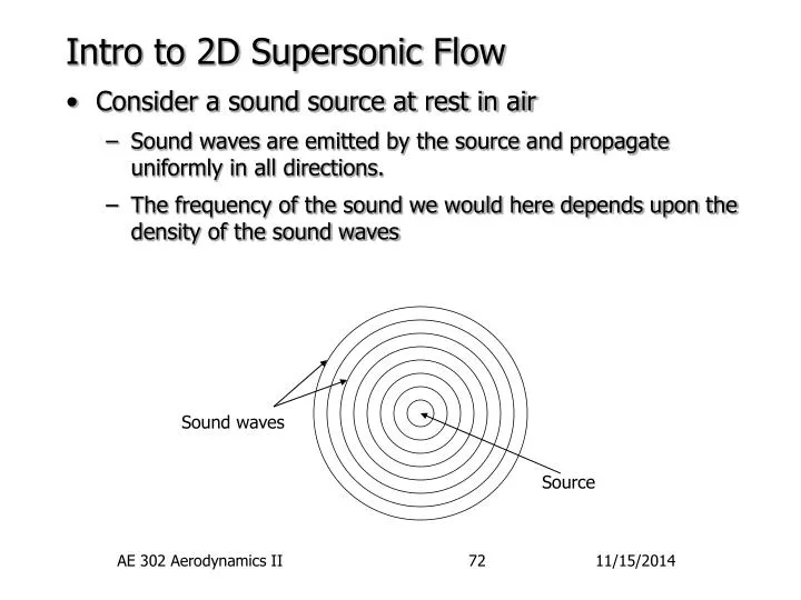
Sound waves. Source. Intro to 2D Supersonic Flow. Consider a sound source at rest in air Sound waves are emitted by the source and propagate uniformly in all directions. The frequency of the sound we would here depends upon the density of the sound waves. Expanded wave pattern,

E N D
Sound waves Source Intro to 2D Supersonic Flow • Consider a sound source at rest in air • Sound waves are emitted by the source and propagate uniformly in all directions. • The frequency of the sound we would here depends upon the density of the sound waves AE 302 Aerodynamics II
Expanded wave pattern, lower frequency sound Compressed wave pattern, higher frequency sound Source moving with subsonic velocity Intro to 2D Supersonic Flow [2] • Now put the sound source into a slow motion to the left: • Because the speed of the wave is independent of the speed of the source, we see the waves bunching up in front. • The frequency of the sound is no longer uniform in all directions, but varies from in front to behind AE 302 Aerodynamics II
Wave front Zone of noise Zone of silence Source moving with supersonic velocity Mach Waves • If we increase the source speed to supersonic: • Source is now moving faster than the sound it emitted • A wave front is formed from the locus of sound waves: only behind this wave front is the source heard. • This wave front has another name: a Mach wave AE 302 Aerodynamics II
Mach wave at Vt Source moving with supersonic velocity Mach Waves [2] • The angle the Mach wave makes with the source velocity vector is called the Mach angle, . • By using the length of the two velocity paths we see that: AE 302 Aerodynamics II
Oblique shock wave M1 > M2 b q =turning angle V Oblique Shock Waves • A Mach wave is the very weak form of a more interesting phenomena, the oblique shock wave. • Oblique shock waves form when a flow turns into itself. They act to turn the flow parallel to the surface and slow it down. • The angle of an oblique shock wave is given the symbol and is always greater than . AE 302 Aerodynamics II
Expansion Fan M1 < M2 m V q =turning angle Expansion Fans • The opposite of an oblique shock wave is called an expansion fan. • Oblique shock waves form when a flow turns away from itself. They also act to turn the flow parallel to the surface but this time they speed it up. • The expansion fan is actually made up of a series of Mach waves – thus it does not produce abrupt flow changes. AE 302 Aerodynamics II
Shock Wave Oblique Shock Relations • Let’s first develop relations for oblique shocks before tackling expansion fans. • What we want to find are the post-shock conditions as well as the shock wave angle. • As before, assume we know all the conditions before the shock. • In addition, we will know what the disturbance is – i.e. the value of the turning angle, . AE 302 Aerodynamics II
Oblique Shock Relations [2] • Begin by selecting a control volume (C.V.) on which to apply our flow conservation equations. • While any C.V. will work, one with side tangent and normal to the shock, as shown, is convenient. • The initial and final velocities for this case have tangent and normal components: AE 302 Aerodynamics II
Oblique Shock Relations [3] • Now apply conservation of mass. • Note that due to symmetry, the in- and out-flow fluxes in the tangent direction cancel each other. • Thus, there are only normal contributions: • Next, apply momentum conservation, which in vector form is: AE 302 Aerodynamics II
Oblique Shock Relations [4] • This needs to be split into tangential and normal equations. • To get the tangential equation, dot the vector equation with the j normal vector: • Thus, the tangential velocity doesn’t change across the shock. • This result may have been logically anticipated since there is no pressure gradient in the tangent direction. AE 302 Aerodynamics II
Oblique Shock Relations [5] • To get the normal momentum equation, dot the vector equation with the i normal vector: • And finally, apply energy conservation: • As with the earlier terms, only the terms involving the normal fluxes don’t cancel. AE 302 Aerodynamics II
Oblique Shock Relations [6] • The result is thus: • Or, after rearranging and apply our mass conservation result: • This equation actually applies to all adiabatic flows. • Another form which is useful can be found by expansion: AE 302 Aerodynamics II
Oblique Shock Relations [7] • But since the tangential velocity doesn’t change, this is just: • So, to summarize all the results: • But note that these last 3 equation are exactly like the normal shock equations – with the normal velocity replacing the x velocity component. • Thus, we can use our previous shock jump results by just inserting the normal Mach number. AE 302 Aerodynamics II
Oblique Shock Jump Equations • Using the normal Mach number, M1n = M1sin, we can write the oblique shock jump equations as either: • We can also use the shock jump tables – as long as M1nis used when looking up values. • But, that means we still need to know first! AE 302 Aerodynamics II
Shock Wave Angle • To find the shock wave angle, use the following geometric relations: • Applying these to the velocity jump equation: • And, after using some trig identities…and a lot of work…this becomes: AE 302 Aerodynamics II
Shock Wave Angle [2] • Unfortunately, this equation expresses as a function of – the opposite of what is useful. • Since this function is non-linear, it cannot be inverted – instead we rely upon the plot. • Pages 513-514 show the plot - -M diagram for air copied from pages 42-43 of NACA Report 1135. AE 302 Aerodynamics II
q < qmax Results from - -M Diagram • At any given Mach number, there is a maximum turning angle, max, with a solution for . • If the body turning angle is greater than max then a “detached” shock is formed. • The detached shock is normal at the wall – giving subsonic flow which can make the turn. • Detached shock are VERY difficult problems to solve – in fact I think you need CFD to do it. q > qmax AE 302 Aerodynamics II
Results from - -M Diagram [2] • For any given q < qmax, there actually two possible solutions! • The lower solution is called the “weak” solution and is the one observed in almost all external flows. • The upper solution is called the “strong” solution. However, this solution is unstable and doesn’t normally occur except in some internal flow situations. • For any initial Mach number M1, the two solutions correspond to: • A normal shock for the strong solution. • A Mach wave for the weak solution, with AE 302 Aerodynamics II
Results from - -M Diagram [3] • The chart shows the line of solutions for M2=1.0. • All the strong solution result in subsonic flow behind the shock. • Almost all the weak solutions have M2>1, i.e. supersonic flow behind the shock! • There are a few weak solutions, all around qmax which result in subsonic flow behind the shock. AE 302 Aerodynamics II
2b bu qu 2q ql bl Wedge and Cone Flow • The previous results for a wall with ramp can also be applied to the flow over a wedge. • The upper and lower surfaces form independent flow solutions divided by the wedge tip: • Thus, we can apply our oblique shock relations to each surface independently using the local turning. • Hovever, note that if q > qmaxon one side – the shock detaches on both!. ql > qmax AE 302 Aerodynamics II
2b 2q B-B A-A Wedge and Cone Flow [2] • If the body is axisymmetric, i.e. a cone, rather than a wedge, the flow looks the same - but takes on a very different character. • To see this consider sectional cuts of the flow at two locations: • A streamtube of air next to the surface has a growing circumference as it goes down stream. B-B A-A AE 302 Aerodynamics II
Wedge and Cone Flow [3] • To conserve mass, the tube thickness decreases to give close to the same flow area at all locations. • Thus, stream lines asymptotically approach the surface of the cone – unlike the wedge where streamlines are tangent to the surface. • Between the shock and the cone, the flow goes through a smooth,isentropic turning and compression. • Since the initial turning angle for cone flow is less than for a wedge, the shock must be weaker – and has a angle closer to m. AE 302 Aerodynamics II
Line of constant flow property Wedge and Cone Flow [4] • As it turns out, rather than have constant flow properties behind the shock as in 2-D – the properties are constant along rays from the apex: • This observation is one of the basis for conical flow theory – and approximate method for solving 3-D flows over wings and fuselages. • Unfortunately, that theory is beyond the scope of this class. AE 302 Aerodynamics II
M1 T1 p1 M2 T2 p2 m2 m1 q Prandlt-Meyer Expansion Waves • Now let’s return to the functional opposite of an oblique shock wave – the expansion fan. • From experimentation, it had already been observed that expansion fans: • Turn the flow to be tangent to the surface • Accelerate the flow while T and p decrease • Are isentropic – total pressure and density are constant. • Prandlt and Meyer were the first to derive a theory for this flow, so it is often called a Prandlt-Meyer expansion. AE 302 Aerodynamics II
M1 T1 p1 M2 T2 p2 m2 m1 q Prandlt-Meyer Expansion Waves [2] • From Schleiren photographs of the flow, it was also known that: • The front edge of the expansion fan is at initial Mach angle from the original flow direction. • The final edge of the fan is at the final Mach angle from the final flow direction. • Thus the fan is made up of weak Mach wave disturbances which smoothly turn the flow from initial to final direction and speed. AE 302 Aerodynamics II
m V dq V + dV Prandlt-Meyer Expansion Waves [3] • Based upon this, the analysis method is to find equations for weak waves that turn the flow by d. • Then, integrate the equations to get the full turning angle . • For a single wave, the geometry shown here gives the relations ship: • Note that the change in velocity is normal to the wave – tangential velocity does not change. AE 302 Aerodynamics II
Prandlt-Meyer Expansion Waves [4] • The previous equation can be re-written as: • And, making a small angle assumption for d, this relation becomes: • Or, if we apply the first term of the power series • This becomes: AE 302 Aerodynamics II
Prandlt-Meyer Expansion Waves [5] • Finally, rearrange this and use the Mach angle definition to get: • This is the function that will be integrated to get the total deflection: • To evaluate this integral, a relationship between velocity and Mach number is needed. • The obvious one is of course: AE 302 Aerodynamics II
Prandlt-Meyer Expansion Waves [6] • When differentiated this becomes: or • Thus, a further relationship between Mach number and the speed of sound is needed! • Using one form of the energy equation gives: or AE 302 Aerodynamics II
Prandlt-Meyer Expansion Waves [7] • Differentiating this expression gives: or • Putting this into our earlier equation gives: • So, finally, the integral equation becomes: AE 302 Aerodynamics II
Prandlt-Meyer Function • The previous integral actually has a analytic solution – but a very long messy one. • To simplify it’s evaluation, Prandlt and Meyer introduced a new flow parameter: • This parameter, called the Prandlt-Meyer function, is the angle a flow would have turned through to get to speed, M, if it started at the speed of sound. • The value of v(M), in degrees, is tabulated in the supersonic tables of NACA 1135 – or in Appendix C of the textbook. AE 302 Aerodynamics II
Prandlt-Meyer Function [2] • The function can also be evaluated analytically as: • The value of this new function comes from splitting the integral for t: • Thus, the turning angle is just the difference between final and initial P-M functions: • Or, even better, the final P-M function (and thus M2) can be found from the initial value and the turning angle: AE 302 Aerodynamics II
Property Changes across a P-M Expansion • One final note. Since the flow across an P-M expansion is isentropic, our previous isentropic flow relations can be used. • Thus, across a P-M expansion: AE 302 Aerodynamics II
Wave Families • The next topic for discussion is wave reflections and interactions. • However, before doing that, it is useful to present a way of classifying waves into families. • If a wave runs to the left as you follow it down, it is in the family of left running waves. • If a wave runs to the right as you follow it down, it is in the family of right running waves. AE 302 Aerodynamics II
M1 M3 M2 M2 M1 M3 Solid Wall Reflections • A wave will reflect off of a solid wall as a wave of the same type, but opposite family. • Thus a left running shock reflects as a right running shock. • Note: this assumes that M2 > 1. • Or, a right running expansion reflects as a left running expansion. AE 302 Aerodynamics II
Solid Wall Reflections [2] • Note that these are not specular (i.e. mirror like) reflections – the reflective wave is not at the same angle as the incident wave. • Instead, the wave strength (and thus its angle) is determined by the requirement of flow tangency to the surface. • Since the turning angles for each wave are the same magnitude then: • For a shock reflection, M1 > M2, therefore, 1 < 2., and the reflection is steeper then the original wave. • For an expansion reflection, M1 < M2, therefore, 1 > 2, and the reflection is shallower then the original. AE 302 Aerodynamics II
M2 M1 M3<1 Mach Reflection • The previous result is only valid as long as < max for the reflection shock as well as the incident one. • For some cases, the Mach number after the first shock is so low that it can no longer turn as far. • In this case, the incident wave turns normal to the wall in what is called a Mach reflection. • The normal shock produces locally subsonic flow on the wall – thus this is a transonic flow problem. AE 302 Aerodynamics II
U M2U M3U M1 M3L M2L L Opposite Family/Same Type Intersections • If two wave of opposite families, but the same type, intersect they reflect off each other as waves of the same type, but opposite family. • Thus, if there is an inlet with ramps on upper and lower walls, the flow looks like: • The strength of the reflected waves is determined by two requirements in region 3: • The two flows must be tangent to one another. • The two flows must be at the same pressure! AE 302 Aerodynamics II
Opposite Family/Same Type [2] • If the flow is isentropic, i.e. expansion or Mach waves, the upper and lower flows would just have to turn back horizontal. • This is not true for shocks, however, due to the total pressure losses (entropy increases). • Instead, the two final flows end up slightly inclined from the horizontal – and the two velocities will not be the same. • The border between upper and lower flow – with an entropy and thus velocity jump is called a slip line. p3 V3U slip line V3L p3 AE 302 Aerodynamics II
M4 M1 2 M3 M2 1 Same Family/Same Type Intersection • If two wave of the same family and the same type intersect they combine to produce a stronger wave of the same type and family. • This can be visualized as the case where a ramp with two increasing angles is used: • Note that there is no corollary for expansion waves since they always turn away from each other! • The two shock waves will always converge due to both the initial ramp angle and the lower value for M2 (higher 2). AE 302 Aerodynamics II
M4 M1 slip line M2 M3 weak reflection Same Family/Same Type Intersection [2] • Where the two waves coalesce into one, the same requirements as before exist: flow tangency and equal pressures. • To meet these requirements, a weak reflected wave comes off the junction – usually an expansion. • Also, a slip line again forms due to the different histories of the two flow paths. • In practice, it is usually sufficient to assume the flow above the junction turns by the total turning angle, . AE 302 Aerodynamics II
Isentropic Compression Ramp • An interesting situation arises when a ramp is used which has a smooth curve – or lots of small steps. • However, a shock will still form away from the surface where the Mach waves eventually coalesce. • The flow in this case is turned by a series of very weak compression waves. • As a result, the flow along the surface may be isentropic – or very close to it. AE 302 Aerodynamics II
M >1 Shock-Expansion Theory • Now that all the preliminary concepts are in place, let’s turn to a practical application – the calculation of forces on an airfoil • We will make two restrictions: • First, there cannot be any detached shocks, and the flow must remain supersonic. • The Mach number must be low enough that wave interactions away from the surface can be neglected. • The 2-D airfoil analysis performed is called Shock-Expansion theory – because the method uses the shock jump and P-M expansion results we just learned. AE 302 Aerodynamics II
y,Fy pu l M x,Fx d pl Shock-Expansion Theory [2] • To calculate the surface pressures, use the appropriate equations for the type and family of wave being generated. • To calculate the lift and drag per unit span, the pressures must be integrated over the chord. • To do this, it is usually easier to integrate to find the forces normal and tangent to the chord line. AE 302 Aerodynamics II
Shock-Expansion Theory [3] • The integral equations are: • And, rotating into the flow direction gives: • Of course, for simple geometries, these equations become simpler also. AE 302 Aerodynamics II
pu pl pl p pu x/c 1.0 Shock-Expansion Theory [4] • For, example, on a flat plate airfoil (dy/dx=0): • This drag – which wouldn’t occur in subsonic flow is what we call wave drag. • Since the pressures, and thus difference in pressures, is constant, the center of pressure is the mid chord, x/c=0.5. AE 302 Aerodynamics II
pu,1 pu,2 2 t pl,1 pl,2 pl,1 pu,1 p pl,2 x/c pu,2 Shock-Expansion Theory [4] • For the diamond, or double wedge, airfoil, the pressures are piecewise constant: • Note that the thickness is related to the wedge angle by: • However, the center of pressure is still at the mid- chord! 1.0 AE 302 Aerodynamics II
Thin Airfoil Theory • The previous method can become rather tedious for complex geometries. • However, it is an “exact” method and must be used if there are strong shocks present. • However, most airfoils are thin and fly at low angles of attach at supersonic Mach numbers. • Thus, it is natural to see if there is an approximate method suitable for weak shocks and nearly isentropic flow. • This method is called Thin Airfoil Theory. AE 302 Aerodynamics II
Thin Airfoil Theory [2] • To develop this method, start with the weak Mach expansion equation derived earlier: • First, let’s generalize this equation to also allow for weak compressions. • To do this, we need to standardize our angles such that an compression turn is positive, an expansion turn is negative: • Next, use Euler’s momentum equation: AE 302 Aerodynamics II