Download
1 / 17
170 likes | 273 Views
Flasher reconstruction. Dima Chirkin, LBNL Presented by Tom McCauley. Reconstruction in fat-reader. fat-reader contains a plug-in reconstruction module, which: uses convoluted pandel description uses multi-media propagation coefficients

E N D
Flasher reconstruction Dima Chirkin, LBNL Presented by Tom McCauley
Reconstruction in fat-reader • fat-reader contains a plug-in reconstruction module, which: • uses convoluted pandel description • uses multi-media propagation coefficients • relies on the Kurt’s 6-parameter depth-dependent ice model • has Klaus’s stability of the solution • parameterization is possible for bulk ice • reconstructs both tracks and showers/flashers • calculates an energy estimate • also reconstructs IceTop showers • New (since the flasher workshop in July): • feature extracts waveforms using fast Bayesian unfolding • corrects the charge due to PMT saturation • accounts for the PMT surface acceptance • combines energy with positional/track minimization
Bayesian waveform unfolding • fast waveform feature extraction: 2-3 ms per every WF (cf. 30 seconds before) • why not invert against the tabulated smearing function • need to emphasize SPE signal while controlling oscillations of the solution due to noise • Bayesian or regularized unfolding does just that
Simple and complicated waveforms are reconstructed with the same amount of effort Bayesian waveform unfolding If a fitted pulse does not start on the boundary, then it is approximated by a superposition of 2 pulses. The weighted average of these pulses gives the estimate of the leading edge.
Energy reconstruction • Before continuing, reminding of the energy estimate: • constructed according to the Rodin’s Monin formula, with average propagation length obtained from average absorbtion and scattering. These are averaged, as during the positional reconstruction, using George/Mathieu prescription based on Kurt’s ice model
From Bai’s DOM test report Measured between 700 and 1750 V PMT saturation As measured by Chiba group at 1.17.107 Qcorr=Q/(1+Q/Qsat) Qsat=7500 (gain/107)-1.24 may require new calibration type?
After the correction for saturation DOMs 29 and 28 turn out to receive 11700 and 5100 PEs PMT saturation in flasher data DOM 30 flashing at 127 FFF 20 ns DOMs 29 and 28 show approx. 4600 and 3070 PEs
OM angular sensitivity From Ped’s thesis, at the moment as parameterized for an AMANDA OM
PMT saturation and OM sensitivity saturation sensitivity
From Gary’s talk: usual hit positional/timing likelihood energy density terms Energy reconstruction From Chrisopher W. reconstruction paper: Therefore, w=1
Combined positional/energy reconstruction • Improves positional reconstruction by constraining the energy observable: • Systematic position offset is less than 5 meters • Estimated event time is close to 0 (cf. ~-100 ns previously)
Energy estimate • It appears that: • the same hierarchy holds throughout depths: in observed energy increasing order: FFF/064 FC0/127 03F/127 FFF/127 • 03F/127 setting is most depth-independent
Energy measurement uncertainty Measured as the RMS of the distribution of energy estimates by all DOMs in the event (width of the distribution in slide 9)
DOM-to-DOM variation Fixing position according to the geometry file, performing only the energy reconstruction Large variation is likely due to ice layering, not entirely inconsistent with a constant. For 03F/127 one obtains 10^(7.53) ph . area [m2].
Measurement at Chiba PMT effective area Chris Wendt’s estimate: 8 . 109+- 20-50% photons (~56 TeV) per flasherboard at FFF/127(20 ns) Average quantum efficiency = 0.165 Cascade: 1.37 105 photons/GeV PMT area = 492.10 cm2 81 cm2 effective area Nph(03F/127) = 4.2 . 109 photons (for 6 LEDs) Energy = 61 TeV At FFF/127(20ns): 8.4 . 109 photons
Nearby or in clear ice follows expectation from geometry verified Flasher timing information Flashing DOM 10 we can measure arrival time of the first photon at DOMs above and below. Those that form sharp distributions can be used for timing jitter measurement (rms of the ditribution) and geometry verification (mean).
Conclusions and outlook • detailed waveform reconstruction improves positional reconstruction. Now it is more viable to do (much faster) • Energy reconstruction can be done at the same time as positional reconstruction (or separately, fixing position) • PMT saturation and OM angular sensitivity are must be accounted for to explain up/down asymmetry • Number of photons emitted in ice is consistent with lab measurements • Timing precision and geometry are verified • More detailed study of depth-dependent parameters and calibration of the Rodin-Monin formula is needed