Download
1 / 18
230 likes | 458 Views
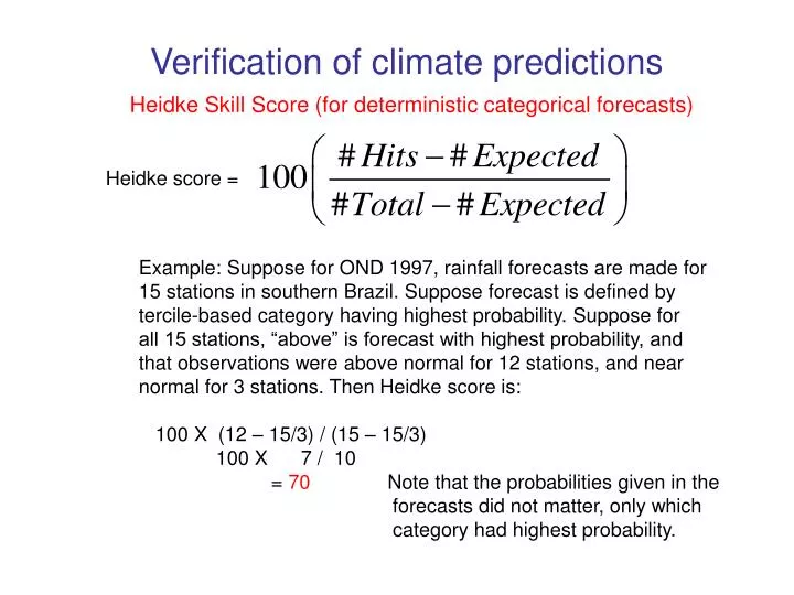
Heidke Skill Score (for deterministic categorical forecasts). Verification of climate predictions. Heidke score = . Example: Suppose for OND 1997, rainfall forecasts are made for 15 stations in southern Brazil. Suppose forecast is defined by

E N D
Heidke Skill Score (for deterministic categorical forecasts) Verification of climate predictions Heidke score = Example: Suppose for OND 1997, rainfall forecasts are made for 15 stations in southern Brazil. Suppose forecast is defined by tercile-based category having highest probability. Suppose for all 15 stations, “above” is forecast with highest probability, and that observations were above normal for 12 stations, and near normal for 3 stations. Then Heidke score is: 100 X (12 – 15/3) / (15 – 15/3) 100 X 7 / 10 = 70 Note that the probabilities given in the forecasts did not matter, only which category had highest probability.
Verification of climate predictions The Heidke skill score (a “hit score”) Mainland United States
Credit/Penalty matrix for some Variations of the Heidke Skill Score O B S E R V A T I O N Original Heidke score (Heidke, 1926 [in German]) for terciles F O R E C A S T O B S E R V A T I O N As modified in Barnston (Wea. and Forecasting, 1992) for terciles O B S E R V A T I O N LEPS (Potts et al., J. Climate, 1996) for terciles
Root-mean-Square Skill Score: RMSSS for continuous deterministic forecasts RMSSS is defined as: where: RMSEf = root mean square error of forecasts, and RMSEs = root mean square error of standard used as no-skill baseline. Both persistence and climatology can be used as baseline. Persistence, for a given parameter, is the persisted anomaly from the forecast period immediately prior to the LRF period being verified. For example, for seasonal forecasts, persistence is the seasonal anomaly from the season period prior to the season being verified. Climatology is equivalent to persisting an anomaly of zero. RMSf =
RMSf = where: i stands for a particular location (grid point or station). fi = forecasted anomaly at location i Oi = observed or analyzed anomaly at location i. Wi = weight at grid point i, when verification is done on a grid, set by Wi = cos(latitude) N = total number of grid points or stations where verification is carried. RMSSS is given as a percentage, while RMS scores for f and for s are given in the same units as the verified parameter.
The RMS and the RMSSS are made larger by three main factors: (1) The mean bias (2) The conditional bias (3) The correlation between forecast and obs It is easy to correct for (1) using a hindcast history. This will improve the score. In some cases (2) can also be removed, or at least decreased, and this will improve the RMS and the RMSSS farther. Improving (1) and (2) does not improve (3). It is most difficult to increase (3). If the tool is a dynamical model, a spatial MOS correction can increase (3), and help improve RMS and RMSSS. Murphy (1988), Mon. Wea. Rev.
Verification of Probabilistic Categorical Forecasts: The Ranked Probability Skill Score (RPSS) Epstein (1969), J. Appl. Meteor. RPSS measures cumulative squared error between categorical forecast probabilities and the observed categorical probabilities relative to a reference (or standard baseline) forecast. The observed categorical probabilities are 100% in the observed category, and 0% in all other categories. Where Ncat = 3 for tercile forecasts. The “cum” implies that the sum- mation is done for cat 1, then cat 1 and 2, then cat 1 and 2 and 3.
The higher the RPS, the poorer the forecast. RPS=0 means that the probability was 100% given to the category that was observed. The RPSS is the RPS for the forecast compared to the RPS for a reference forecast that gave, for example, climatological probabilities. RPSS > 0 when RPS for actual forecast is smaller than RPS for the reference forecast.
Suppose that the probabilities for the 15 stations in OND 1997 in • Southern Brazil, and the observations were: • forecast(%)obs(%) RPS calculation • 1 20 30 50 0 0 100 RPS=(0-.20)2+(0-.50)2+(1.-1.)2 =.04+.25 +.0 = .29 • 2 25 35 40 0 0 100 RPS=(0-.25)2+(0-.60)2+(1.-1.)2 =.06+.36 +.0 = .42 • 3 25 35 40 0 0 100 • 4 20 35 45 0 0 100 RPS=(0-.20)2+(0-.55)2+(1.-1.)2 =.04+.30 +.0 = .34 • 5 15 30 55 0 0 100 • 6 25 35 40 0 0 100 • 7 25 35 40 0 100 0 RPS=(0-.25)2+(1-.60)2+(1.-1.)2 =.06+.16 +.0 = .22 • 8 25 35 40 0 0 100 • 9 20 35 45 0 0 100 • 10 25 35 40 0 0 100 • 11 25 35 40 0 100 0 • 12 20 35 40 0 100 0 • 13 15 30 55 0 0 100 RPS=(0-.15)2+(0-.45)2+(1.-1.)2 =.02+.20 +.0 = .22 • 14 25 35 40 0 0 100 • 25 35 40 0 0 100 • Finding RPS for reference (climatol baseline) forecasts: • for 1st forecast, RPS(clim) = (0-.33)2+(0-.67)2+(1.-1.)2 = .111+.444+0=.556 • for 7th forecast, RPS(clim) = (0-.33)2+(1.-.67)2+(1.-1.)2 = .111+.111+0=.222 • for a forecast whose observation is “below” or “above”, PRS(clim)=.556
forecast(%)obs(%) RPS and RPSS(clim) RPSS • 1 20 30 50 0 0 100 RPS= .29 RPS(clim)= .556 1-(.29/.556) = .48 • 2 25 35 40 0 0 100 RPS= .42 RPS(clim)= .556 1-(.42/.556) = .24 • 3 25 35 40 0 0 100 RPS= .42 RPS(clim)= .556 1-(.42/.556) = .24 • 4 20 35 45 0 0 100 RPS= .34 RPS(clim)= .556 1-(.34/.556) = .39 • 5 15 30 55 0 0 100 RPS= .22RPS(clim)= .556 1-(.22/.556) = .60 • 6 25 35 40 0 0 100 RPS= .42RPS(clim)= .556 1-(.42/.556) = .24 • 7 25 35 40 0 100 0 RPS= .22 RPS(clim)= .222 1-(.22/.222) = .01 • 8 25 35 40 0 0 100 RPS= .42 RPS(clim)= .556 1-(.42/.556) = .24 • 9 20 35 45 0 0 100 RPS= .34RPS(clim)= .556 1-(.34/.556) = .39 • 10 25 35 40 0 0 100 RPS= .42 RPS(clim)= .556 1-(.42/.556) = .24 • 11 25 35 40 0 100 0 RPS= .22 RPS(clim)= .222 1-(.22/.222) = .01 • 12 20 35 40 0 100 0 RPS= .22 RPS(clim)= .222 1-(.22/.222) = .01 • 13 15 30 55 0 0 100 RPS= .22 RPS(clim)= .556 1-(.22/.556) = .60 • 14 25 35 40 0 0 100 RPS= .42 RPS(clim)= .556 1-(.42/.556) = .24 • 25 35 40 0 0 100 RPS= .42 RPS(clim)= .556 1-(.42/.556) = .24 • Finding RPS for reference (climatol baseline) forecasts: • When obs=“below”, RPS(clim) = (0-.33)2+(0-.67)2+(1.-1.)2 =.111+.444+0=.556 • When obs=“normal”, RPS(clim)=(0-.33)2+(1.-.67)2+(1.-1.)2 =.111+.111+0=.222 • When obs=“above”, RPS(clim)= (0-.33)2+(0-.67)2+(1.-1.)2 =.111+.444+0=.556
RPSS for various forecasts, when observation is “above” forecast tercile Probabilities - 0 + RPSS 100 0 0 -2.60 90 10 0 -2.26 80 15 5 -1.78 70 25 5 -1.51 60 30 10 -1.11 50 30 20 -0.60 40 35 25 -0.30 33 33 33 0.00 25 35 40 0.24 20 30 50 0.48 10 30 60 0.69 5 25 70 0.83 Note: issuing too-confident forecasts 5 15 80 0.92 causes high penalty when incorrect. 0 10 90 0.98 Under-confidence also reduces skill. 0 0 100 1.00 Skills are best for true (reliable) probs.
The likelihood score The likelihood score is the nth root of the product of the probabilities given for the event that was later observed. For example, using terciles, suppose 5 forecasts were given as follows, and the category in red was observed: 45 35 20 The likelihood score 33 33 33 disregards what prob- 40 33 27 abilities were forecast 15 30 55 for categories that did 20 40 40 not occur. The likelihood score for this example would then be = = 0.40 This score could then be scaled such that 0.333 would be 0%, and 1 would be 100%. A score of 0.40 would translate linearly to (0.40 - 0.333) / (1.00 - 0.333) = 10.0%. But a nonlinear translation between 0.333 and 1 might be preferred.
Relative Operating Characteristics (ROC) for Probabilistic Forecasts Mason, I. (1982) Australian Met. Magazine The contingency table that ROC verification is based on: | Observation Observation | Yes No --------------------------------------------------------------------------- Forecast: Yes |O1 (hit) NO1 (false alarm) Forecast: NO | O2 (miss) NO2 (correct rejection) --------------------------------------------------------------------------- Hit Rate = 01 / (O1+O2) False Alarm Rate = NO1 / (NO1+NO2) The Hit Rate and False Alarm Rate are determined for various categories of forecast probability. For low forecast probabilities, we hope False Alarm rate will be high, and for high forecast probabilities, we hope False Alarm rate will be low.
| Observation Observation | Yes No --------------------------------------------------------------------------- Forecast: Yes |O1 (hit) NO1 (false alarm) Forecast: NO | O2 (miss) NO2 (correct rejection) --------------------------------------------------------------------------- The curves are cumulative from left to right. For example, “20%” really means “100% + 90% +80% + ….. +20%”. Curves farther to the upper left show greater skill. no skill negative skill Example from Mason and Graham (2002), QJRMS, for eastern Africa OND simulations (observed SST forcing) using ECHAM3 AGCM
| Observation Observation | Yes No --------------------------------------------------------------------------- Forecast: Yes |O1 (hit) NO1 (false alarm) Forecast: NO | O2 (miss) NO2 (correct rejection) --------------------------------------------------------------------------- Hanssen and Kuipers (1965), Koninklijk Nederlands Meteorologist Institua Meded. Verhand, 81-2-15 The Hanssen and Kuipers score is derivable from the above contingency table. Hanssen and Kuipers (1965), Koninklijk Nederlands Meteorologist Institua Meded. Verhand, 81-2-15 It is defined as KS = Hit Rate - False Alarm Rate (ranges from -1 to +1, but can be scaled for 0 to +1). KS When scale the KS as KSscaled = (KS+1) / 2 then the score is comparable to the area under the ROC curve.
Basic input to the Gerrity Skill Score: sample contingency table.
Gerrity Skill Score = GSS = Gerrity (1992), Mon. Wea. Rev. Sij is the scoring matrix Note that GSS is computed using the sample probabilities, not those on which the original categorizations were based (0.333,0.333,0.333). where
The LEPSCAT score (linear error in probability space for categories) Potts et al. (1996), J. Climate is an alternative to the Gerrity score (GSS) Use of Multiple verification scores is encouraged. Different skill scores emphasize different aspects of skill. It is usually a good idea to use more than one score, and determine more than one aspect. Hit scores (such as Heidke) are increasingly being recognized as poor measures of probabilistic skill, since the probabilities are ignored (except for identifying which category has highest proba- bility).