Back to House Prices…

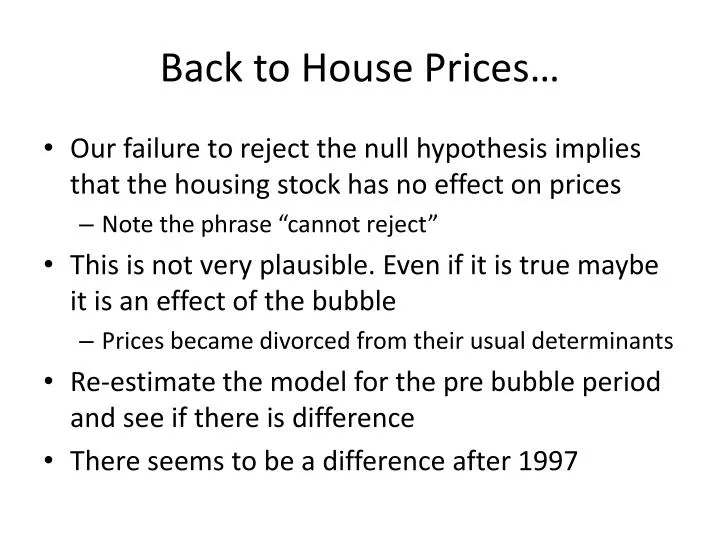
1. Back to House Prices… • Our failure to reject the null hypothesis implies that the housing stock has no effect on prices • Note the phrase “cannot reject” • This is not very plausible. Even if it is true maybe it is an effect of the bubble • Prices became divorced from their usual determinants • Re-estimate the model for the pre bubble period and see if there is difference • There seems to be a difference after 1997

2. Structural Break • This is known as a structural break or a regime shift • Implies that the coefficients may be different not just the variables • So the conditional expectation function has a kink • Can happen at a point in time or for a different group of observations

3. b b Y E(Y|X)= + X 1 2 Y 1 u1 Y u 3 3 Y u 2 2 b 1 X X X X 2 1 3 A Regime Shift Show three data points for illustration

4. House Prices

5. Estimating with Structural Break • Stata command: regress … if condition regress price inc_pchstock_pc if year<=1997 Source | SS df MS Number of obs = 28 -------------+------------------------------ F( 2, 25) = 88.31 Model | 1.1008e+10 2 5.5042e+09 Prob > F = 0.0000 Residual | 1.5581e+09 25 62324995.9 R-squared = 0.8760 -------------+------------------------------ Adj R-squared = 0.8661 Total | 1.2566e+10 27 465423464 Root MSE = 7894.6 ------------------------------------------------------------------------------ price | Coef. Std. Err. t P>|t| [95% Conf. Interval] -------------+---------------------------------------------------------------- inc_pc | 10.39438 1.288239 8.07 0.000 7.741204 13.04756 hstock_pc | -637054.1 174578.5 -3.65 0.001 -996605.3 -277503 _cons | 135276.6 35433.83 3.82 0.001 62299.24 208253.9 ------------------------------------------------------------------------------

6. Interpreting Results • We can reject the null that housing stock has no effect on price • How? Do the details yourself • It has the correct sign i.e. as theory would suggest • We can use this “pre-bubble” model to predict what prices would have been • Use “predict” command • Note this command predicts out of sample also

7. The Pre Bubble Model

8. Interpreting the Graph • Historically house prices have been determined by per capita income and the per capita housing stock. • We estimate the parameters of that relationship before 1997 • If the relationship had remained constant after 1997 prices would have followed the red line • They difference between the two is huge (100% at peak)

9. Interpreting the Graph • So prices rose rapidly even as the stock of houses rose • Note we are not saying that prices should have remained constant • They should have risen in line with income • But the rose by more • If the parameters had remained the same then prices would have followed the red line

10. But the marginal effect of income and stock should have remained the same • Income effect rose (more positive) • Stock effect rose (less negative) • The change in parameters is the structural break that constitutes the bubble • Note: this definition of a bubble would not be universally accepted

11. How Low Will They Go? • If we believe our model then the parameters from pre 1997 still hold • This doesn’t mean that prices will return to 1997 levels • It does mean that prices will return to the level determined by todays income (and stock) using the pre-bubble coefficients • The red line represents the future level of house prices • This represents a decline of 53% from 2010 levels!!!

12. Quality of Prediction • Before we get too confident in this (or any) model it is worthwhile to assess whether it is a good predictor. • We measure this using the R2 (“R-Squared”) and the adjusted R2 • Both of these measure how much of the variation in the Y variable is explained by all the X variables collectively

13. R2 • Let’s look at the model again • Full model: Yi= b0+b1X1i+ b2X2i+ ...+bkXki+ ui • Where E(Y|X)=b0+b1X1i+ b2X2i+ ...+bkXki • uiis the residual • For ease of notation let • So the model can be re-written as • Subtract the sample mean from both sides to get • Note that the sample mean doesn’t have a subscript

14. Now square it and sum over observations to get TSS = ESS + RSS • Total Sum of Squares (TSS) measures the total variation of the Y variable in the sample • Note that the variance would be this divided by N • Explained Sum of Squares (ESS) is the variation that is explained by the model i.e. by the “line” • The Residual Sum of Squares (RSS) is the unexplained portion of the variation in Y • Also know as SSR • Thing we minimized for OLS

15. R2 = ESS/TSS • It gives the proportion of the total variation in the Y variables that is explained by the model • By all the x variables collectively • It doesn’t say anything about which of the X variables are responsible for what portion of the variance • Doesn’t say if the individual coefficients are statistically significant (multicolinearity) • Doesn’t say if the individual coefficients make economic sense • If want to use the model to predict Y then we want R2 to be high • Model explained a lot of the historical variation so it should explain a high proportion of the future variation • i.e. make good predictions • Doesn’t automatically follow that high R2 model is better than lower R2 model

16. Adjusted R2 • Amend formula slightly to account for number of variables • A model with more variables will automatically have higher R2 • Some authors prefer adjusted R2 (also called Rbar squared and denoted by

17. Using either R2 • Compare two different models • Must have same Y variable • Must have the same sample • Be aware that more variables will necessarily lead to higher R2 but not necessarily higher • R2 (either) only tell you how good the model is at predcition • Doesn’t say anything about whether model is economically sensible • For that we need to look at the coefficients