Download

1 / 49
490 likes | 569 Views
How Low Can House Prices Fall?. (Quite a bit). Learning Outcomes. Expand the regression model to allow for multiple X variables Formalise the hypothesis test procedure using test statistics Look at more general hypothesis tests Multiple coefficients Inequality hypotheses

E N D
How Low Can House Prices Fall? (Quite a bit)
Learning Outcomes • Expand the regression model to allow for multiple X variables • Formalise the hypothesis test procedure using test statistics • Look at more general hypothesis tests • Multiple coefficients • Inequality hypotheses • Formalise a procedure for using regression for prediction
House Prices • We all know the story of financial crisis • House price bubble • Banks borrow abroad to finance bubble • Bubble bursts and banks cant get money bank • Bankrupt banks bailed out by state • State bankrupted and bailed out by Troika • See nama.biz if interested
Two Questions • Could we have used econometrics to test for the presence of a bubble? • Now that the bubble is burst, can we use econometrics to say how far have prices to fall? • Yes to both
Immediate relevance • Should you buy or rent now? • How big is remaining hole in the banks? • What about other bubbles? China?
Look at data • Look at aggregate macro time series data of Irish house prices in housing.dta • Stata: line psecd • Certainly a rapid rise • Was it justified? • Incomes and population were rising at the time • By enough? • Econometrics can answer this question
How to Answer the 2 Q • Make use of conditional expectation interpretation of a regression • Recall that regression line gives E(Y|X) • So we will use OLS to give us the expected price of a house conditional on income, population etc • Answers • If the actual price is systematically above the expected price we have evidence of a bubble • After burst the price will fall to the conditional expectation
Extending OLS to Many Xs • We need to understand how OLS works when there are many independent (RHS) variables • Recall: E(Y|X)=b1+b2X • Generalise to: • E(Y|X)=b0+b1X1i+ b2X2i+ ...+bkXki • So the full model becomes: • Yi = b0+b1X1i+ b2X2i+ ...+bkXki+ ui
Interpreting bk • Each parameter 2 , 3 …kmeasures the isolated effect of x2, x3 , xkon the dependantvariable y • Partial Regression coefficients. • In terms of calculus bk is a partial derivative • The effect of changing one variable while keep all others constant
Interpreting OLS • OLS still gives the best line • The only difference is that the “line” isn't a line any more, it is a multi-dimensional hyper plane • The actual data still deviates from the “line” • The “line” is still the conditional expectation • So if confused use the intuition from the single RHS variable case
Intuition of single X case is still valid Show three data points for illustration
Maths of OLS • The formulae for OLS are much more complicated • Really need matrix algebra to write them down • But idea is same • Choose estimates b0 …bk to minimise the sum of squared deviations • Computer does it for us with the regress command
A Preliminary Answer • As with many projects we first need an economic model • Just like Keynes consumption function • Our model will assert that real house prices are a function of per capita real income and the per capita housing stock • Need to generate variables from the raw data Generate • real house prices:gen price=psecd/p*100 • Real per capita income: gen inc_pc=gni/pop*1000 • Real pc housing stock: gen hstock_pc=hstock/pop
OLS Estimates of Model regress price inc_pchstock_pc Source | SS df MS Number of obs = 41 -------------+------------------------------ F( 2, 38) = 210.52 Model | 6.7142e+11 2 3.3571e+11 Prob > F = 0.0000 Residual | 6.0598e+10 38 1.5947e+09 R-squared = 0.9172 -------------+------------------------------ Adj R-squared = 0.9129 Total | 7.3202e+11 40 1.8301e+10 Root MSE = 39934 ------------------------------------------------------------------------------ price | Coef. Std. Err. t P>|t| [95% Conf. Interval] -------------+---------------------------------------------------------------- inc_pc | 16.15503 2.713043 5.95 0.000 10.66276 21.6473 hstock_pc | 124653.9 389266.5 0.32 0.751 -663374.9 912682.6 _cons | -190506.4 80474.78 -2.37 0.023 -353419.1 -27593.71 ------------------------------------------------------------------------------
Predicting Prices • We can use this model to predict prices • Recall that OLS gives us an estimate of the conditional expectation function • Put in the numbers • E(Y|X)=b0+b1X1i+ b2X2i+ ...+bkXki • E(Price|inc_pc, hstock_pc)=-190506.4 + 124653.9*hstock_pc+ 16.15503*inc_pc
Predicting Prices • We can use generate command to create a variable with this conditional expectation • gen pred=-190506.4 + 124653.9*hstock_pc+ 16.15503*inc_pc • So useful there is a special command • predict pred • Compare the two on a graph • line price pred year
Interpretation • The predicted line is our estimation of what we would expect the price to be given the level of income and the housing stock • The actual price was systematically above this expected price from 2003 • This could be seen as evidence of a bubble • Note how it fits in to the discussion of the time which said that prices went up but this was justified given the rise in incomes • We show that prices went up more than we would “expect” for the observed increase in incomes • So we show that prices too high in a precise sense
More can be done • We can test hypotheses about the variables to see if they have effects consistent with theory • If the effects were different from our preconceived notions we may be wary of trusting the estimates • i.e. we got a fluke sample
Housing Stock Has no Effect? • Test the null hypothesis that housing stock has no effect on prices H0: bH= 0 H1: bH≠0 • Calculate the distribution of bOLS assuming that H0 is true. • Find our estimate on the distribution • What is the probability that our estimate would have come from this distribution? • Does this lead us to believe the null hypothesis?
Quite possible to get an estimate of 124653.9 if the true value is 0.0 • Note that this has nothing to do with the scale of the estimate. The estimate is a big number but it is not statistically different from zero. • Calculate the probability • P(bOLS≥124653.9| bH=0.0)= • P(z ≥(124653.9-0)/(389266.5)) • P(z ≥0.32)= 0.37 • Clearly this is much larger than usual threshold values of 5%,10% or 1% • So we cannot reject the null hypothesis
Comments • We could reject the null if our threshold was 40% • Seems very extreme • Think of criminal trial metaphor • Cannot reject idea that effect of housing stock is zero even though the estimated effect is 120000! • Scale of coeff has NO impact on statistical significance • Result does seem unlikely as contradicts theory • How to resolve this contradiction? • Look carefully at both theory and estimates • Sniff test! • Can simplify test procedure
Test Statistics • Clearly a large degree of commonality between our tests even though they were on different data • So we can systematize things a little better • The key part of each test was calculating Z using one of the key properties of normal distributions
So now we only ever have to deal with one distribution, the “standard” normal • The two diagrams correspond but the z distribution will be the same every time • Note also how the construction of Z explicitly removes the issue of scale • Stn err has same scale as coeff. • Stream-lined Test procedure • State Hypothesis • Calculate Z assuming H0 is true • Now we can compare the calculated values of Z with the standard normal distribution
The Housing Stock Example • State the Hypothesis we want to test H0: bH= 0 H1: bH≠ 0 • Calculate the test statistic assuming that H0 is true. z =(124653.9-0)/(389266.5)=0.32 • Find our estimate on the distribution • Either find the test statistic on the standard normal distribution • Or compare with one of the traditional threshold (“critical”) values: 2.58(1%), 1.96 (5%), 1.64(10%) • |Z|<all the critical values • So we cannot reject the null hypothesis
Comment • We will reject the idea that bH= 0.0 if there is overwhelming evidence that bHis bigger or smaller • The evidence is our estimate (120000) • Is this big enough? It looks huge • But the standard error is huge also – so a very wide distribution of estimates • So probability of a large estimate arriving by fluke is high • Remove the scale from the problem by calculating the test statistic: Z=0.32
Comment • Is this big enough? • Traditionally 1.96 would be the “critical value” because of 5% probability of |Z|>1.96 as fluke • “beyond reasonable doubt” • Free to decide for ourselves (p-value) • p-value=Pr(|Z|>0.32)=0.75
Issues in Hypothesis Testing • Test of significance • “t-test” • Rule of thumb • General procedure • Significance level • P-value
Test of Significance • A test of H0: b= 0 is given the special name of “test of significance” • Test statistic is simple Z=(bOLS – b)/se(bOLS)= bOLS/se(bOLS) Which is calculated by most statistical software • Simple eyeball test of significance • Variable is or is not “statistically significant” • Not the same as economically significant
t-test • Strictly speaking the Z test is only valid when s, the variance of u is known as it is used to calculate se(b) • s will almost never be known and will have to be estimated • When it is estimated the distribution of the estimator (and therefore the test statistic) is no longer normal • Has a t-distribution • Typically thicker tails than normal. Why?
t-test • The precise shape of the t distribution depends on degrees of freedom: N-K • N is number of observations • K is the number of variables • So the critical values will vary with N-K • Fortunately t≈Z when N-K is large • Stata reports t-test for statistical significance automatically (see over)
OLS Estimates of Model regress price inc_pchstock_pc Source | SS df MS Number of obs = 41 -------------+------------------------------ F( 2, 38) = 210.52 Model | 6.7142e+11 2 3.3571e+11 Prob > F = 0.0000 Residual | 6.0598e+10 38 1.5947e+09 R-squared = 0.9172 -------------+------------------------------ Adj R-squared = 0.9129 Total | 7.3202e+11 40 1.8301e+10 Root MSE = 39934 ------------------------------------------------------------------------------ price | Coef. Std. Err. t P>|t| [95% Conf. Interval] -------------+---------------------------------------------------------------- inc_pc | 16.15503 2.713043 5.95 0.000 10.66276 21.6473 hstock_pc | 124653.9 389266.5 0.32 0.751 -663374.9 912682.6 _cons | -190506.4 80474.78 -2.37 0.023 -353419.1 -27593.71 ------------------------------------------------------------------------------ T-test of statistical significance P-value of the T-test
Rule of Thumb • Easy to “learn off” test procedure • calculate the test statistic • Reject hypothesis if test statistic>2 in absolute terms • Useful for “eyeball” tests of significance • Works because most critical values are below 2 • Stata command “test” does the whole procedure automatically • But does “F-test” • This is the square of t-test
T-Test of Two sided Hypotheses • State the null and alternative hypothesis • H0: b= c H1: b= c • Note when the hypothesis is “two sided” the null be rejected if estimate is very big or very small • Choose a significance level i.e. the threshold for rejection (denoted by a) • 1%, 5%, 10% or another • Free to choose but there are consequences (later) • Calculate the test statistic • T=(b-bH)/se(b)
Find the test statistic on the distribution Two methods Hint: always helps to draw the distribution • The Critical Value method • Find the critical values on the distribution. Look up tables and/ or stata • You will need significance level and degrees of freedom • The +/- critical values define rejection region • Reject null if in the rejection region i.e. if the test statistic is greater than the critical value in absolute terms
The P-value method • Find the probability that a draw from the distribution of the test static would be greater in absolute terms than the actual value of the test statistic observed • The p-value is twice this calculated value • Reject the null if p<a • Clearly state the result noting the significance level • This is very important • Can reject at one a and fail to reject at another
The Housing Stock Example Again • H0: bH= 0 H1: bH≠0 (clearly two sided) • Significance level: choose 1% 5% 10% • Calculate the test statistic assuming that H0 is true. t=(124653.9-0)/(389266.5)=0.32 • Find our estimate on the distribution • Critical value method • Df=41-3=38: SL 1,5,10 use stata command: diinvttail(38,0.005) • Or look up tables • Critical values are : 2.71; 2.02; 1.68 (hint: check makes sense on diagram) • T-stat is less than all the critical values for all significance level • P-value method • Pr(|t|>032)=pr(t>0.32)+pr(t<-0.32)=2*pr(t>0.32) • Stata command: dittail(38,0.32) • P value is 0.75 • P>alpha • So we cannot reject the null hypothesis at the 1%, 5% or 10% significance levels
Comments and Hints • Always draw the diagram and label it clearly • Check on the diagram that higher critical values correspond to lower significance level • Both imply smaller rejection region, so less likely to reject • Remember these tests are two sided • Two regions each with half the significance level • Careful when looking up the critical values • Why? We can reject if extremely small or large t
Up to you whether use critical value method or p-value method • Critical value easier initially • P value more common now because of computers • Need to understand both • Always indicate the significance level that you are working with • Crucial for exam • You are free to choose a • Certain values are typically used but this is convention • One reason for popularity of p-values, can see instantly at what a you would reject
Choosing Significance Level • Roughly: Probability of a fluke • When we choose a critical value we choose a significance level also: • 2.58(1%), 1.96 (5%), 1.64(10%) for large df • If we reject the null because |t|>1.96, we say we reject the null at the 5% significance level. • We acknowledge that there is a 5% chance that t>1.96 even though the null is true • This is type 1 error: Rejecting a true Null • Criminal trial: Convicting the innocent
The test is set up make this as low as possible • i.e. reject only if overwhelming evidence • Why not make it zero? Cant because would never reject any null • Criminal: always acquit • Type II error: fail to reject a false null • All This matters because setting up a hypothesis is setting up a procedure that is deliberately biased against rejecting • Compare the size of rejection region • Make sure that is what you want for your null