Download
1 / 34
370 likes | 647 Views
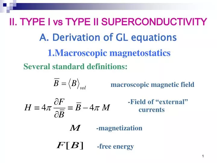
A. Derivation of GL equations. II. TYPE I vs TYPE II SUPERCONDUCTIVITY. 1.Macroscopic magnetostatics. Several standard definitions:. macroscopic magnetic field. -Field of “external” currents. -magnetization. -free energy.

E N D
A. Derivation of GL equations II. TYPE I vs TYPE II SUPERCONDUCTIVITY 1.Macroscopic magnetostatics Several standard definitions: macroscopic magnetic field -Field of “external” currents -magnetization -free energy
In equilibrium under fixed external magnetic field the relevant thermodynamic quantity is the Gibbs energy: Inserting the GL free energy: one obtains:
2. Derivation of the LG equations By variation with respect to order parameter Y one obtains the nonlinear Schrodinger equation and by variation with respect to vector potential A - the supercurrent equation out of five equations only four are independent (local gauge invariance)
The equations should be supplemented by the boundary conditions. The covariant gradient is perpendicular to the surface (*) while the magnetization is parallel to it: (**) Note that the external magnetic field enters boundary conditions only – magnetic field is a “topological charge”.
Details of the derivation of the set of GL equations and boundary conditions We have to vary with respect to five independent fields: and Two components of the complex order parameter field are varied independently. One of them is:
If the full variation dG is to vanish, one has to require that both the nonlinear Shroedinger eq. and the boundary condition (*) are satisfied. Variation with respect to Y(x) just gives the corresponding complex conjugate equation.
This defines supercurrent The covariant derivative representation makes its gauge invariance obvious. The variation of is identical to that used in derivation of Maxwell equations.
This leads to the supercurrent equation and the boundary condition (**) .
The boundary condition (*) after multiplication by the order parameter field leads to Supercurrent therefore cannot leave the superconductor through theboundary and therefore circles inside the sample.
B. Homogeneous and slightly perturbed SC solution 1. Zero magnetic field. Homogeneous solutions. The degenerate minima are at with free energy density
The condensation energy In addition to the degenerate SC solution (global minima) there exists a nondegeneratetrivial normal solution (a local maximum): The free energy density difference between the normal and the superconducting ground states (the condensation energy) is: where Hc is defined as the “thermodynamic critical field”. As will be clear later at this field nothing special happens in type II superconductor.
2. A small inhomogeneity near the SC state Deviations of the order parameter Assume that variations are along the x direction only and the magnetic field contributions are small : Is real Defining the normalized order parameter
one is left with a single scale the coherence length For small deviations of from one linearizes the (anharmonic oscillator type) equation with
This corresponds to the “harmonic approximation”. Deviations of from decay exponentially on the scale of correlation length
The magnetic field penetration profile In the supercurrent equation the magnetic field cannot be neglected. However in this case one can neglect setting This is the Londons’ equation, valid beyond GL theory, everywhere close to deep inside the superconductor. Taking a curl, one obtains:
The relevant scale here is the penetration depth The solution of the linear Londons’ eq. is also exponential: The magnetic field decays exponentially inside superconductor on the scale of magnetic penetration depth.
Anderson – Higgs mechanism In unitary gauge (and absence of topological charge=flux) order parameter Ycan be made real
In harmonic approximation one expands to second order around the SC state and obtains (up to a constant) following quadratic terms (linear terms generally vanish due to eq. of motion or GL eqs.):
In the normal phase one has three massless excitation fields: two transverse polarizations of photon (use, for example the Colomb gauge and the phase of order parameter In the SC phase the situation changes dramatically: due to “mixing” all the excitations become massive. In the unitary gauge this is seen as a three component massive vector field A. The situation is sometimes termed “spontaneous gauge symmetry breaking”.
Type II large k l > x Type I small k x > l SC N SC N x l l x sinterface > 0 sinterface < 0 Beyond perturbation theory Of course when deviations are not small like in the SC-N junction one has to consider both the order parameter and the magnetic field simultaneously and go beyond the perturbation theory.
Gn Gs superconductor normal C. The SC-normal domain wall surface energy. • Extreme type II case: the energy gain due to magnetic field penetration into SC Assume first In the SC region but
The Gibbs free energy density in the N part (assuming ) is the same as is homogeneous SC On the SC side assume that one still can use the Londons asymptotics with : The energy gain is therefore: Highly unusual!
Gn Gs super normal 2. Extreme type I limit: the energy loss due to order parameter depression near N In the opposite case In the junction region but The energy loss of the condensation energy naively is: Less naively one solves the anharmonic oscillator type equation exactly:
Details of solution Multiplying the eq. by and integrate over x with boundary conditions one obtains
Therefore in type I SC the behavior is as expected: one has to pay energy in order to create interfaces. Summing up naively the two contribution we obtain the interface energy For the domain wall energy changes sign. Type II SC unlike any other material, likes to create domain walls.
3. General case A convenient choice of gauge for the 1D problem: Set of GL equations (the solution Y(x) is real) is or using dimensionless functions and
Using l(T)as a unit of length this becomes The boundary conditions still are:
A simplified expression for the domain wall energy Nonlinear Schrodinger equation simplifies the expression: Exercise 1: solve the GL equations for S-N numerically using the shooting method fork=.5,1,10.
4. For what k the interface energy vanishes? Obviously s in (*) vanishes if the integrand vanishes It turns out that for the exact solution (which is not known analytically) obeys it! For this particular value of k the GL equations (with x in units of l) takes a form:
Substituting the zero interface requirement (*) into the second eq.(2) one gets: Differentiating it and using (*) again one gets eq.(1): The value therefore separates between type I and type II.
Summary 1. Order parameter changes on the scale of coherence length x, while magnetic field on the scale of the penetration depth l. The only dimensionless quantity is k=l/x. 2. The interface energy between the normal and the superconducting phases in type II SC is negative. This leads to energetic stability of an inhomogeneous configuration. 3. The critical value of the Ginzburg parameter kat which a SC becomes type II is