Download
1 / 23
340 likes | 725 Views
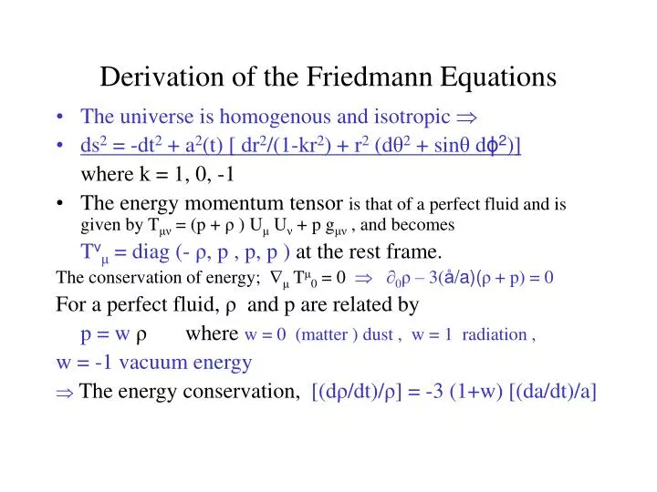
Derivation of the Friedmann Equations. The universe is homogenous and isotropic ds 2 = -dt 2 + a 2 (t) [ dr 2 /(1-kr 2 ) + r 2 (d θ 2 + sin θ d ɸ 2 )] where k = 1, 0, -1

E N D
Derivation of the Friedmann Equations • The universe is homogenous and isotropic • ds2 = -dt2 + a2(t) [ dr2/(1-kr2) + r2 (dθ2 + sinθ dɸ2)] where k = 1, 0, -1 • The energy momentum tensor is that of a perfect fluid and is given by Tμν = (p + ρ ) Uμ Uν + p gμν, and becomes Tνμ = diag (- ρ, p , p, p ) at the rest frame. The conservation of energy; μ Tμ0 = 0 0ρ – 3(å/a)(ρ + p) = 0 For a perfect fluid, ρ and p are related by p = w ρ where w = 0 (matter ) dust , w = 1 radiation , w = -1 vacuum energy The energy conservation, [(dρ/dt)/ρ] = -3 (1+w) [(da/dt)/a]
The Einstein Equations, Rμν – (1/2) gμν R = 8π GNTμν or Rμν = 8π GN ( Tμν - (1/2) gμν T ) results in Friedmann Equations: μν = 00 (ä/a) = -(4π GN /3)(ρ + 3p) μν = ij (å/a)2 = (8π GN /3)ρ – (k/a2) (å/a) : Hubble parameter The observation of the acceleration of the expansion of the universe implies (ä/a) > 0 , that is, most of the dark energy is in the form of vacuum energy i.e. cosmological constant
A symmetry for vanishing cosmological constant Recai Erdem, 2006
The Theoretical Source of theCosmological Constant • Einstein field equations:Rμν – (1/2) gμν R = 8GNTμν - gμνΛ ( i.e gravitational action: IG = (1/ 8GN)-g d4x (R - Λ) + -g d4x ℒ ) Λ: cosmological constant energy density with the energy-momentum tensor Tμν= - gμνρ , ρ = Λ /(8GN) (with positive energy density and negative pressure for Λ>0) ρcan be considered as a vacuum energy density ρ = <ℒ>.
Motivation for studying Cosmological Constant • A conservative candidate for a dark energy (component) with a repulsive force to explain the accelerated expansion rate of the universe a positive Cosmological Constant • Any contribution to the vacuum energy (e.g. vacuum polarization in quantum field theory) contributes to the cosmological constant
Cosmological Constant Problems • 1-Why so huge discrepancy between the observed and the theoretical values of Λ? (Λtheoretical /Λexperimetal ) ~ 1041 – 10118 Due to zero-point energies in chromodynamics ~ 1041 - Due to zero-point energies in gravitation at Planck scalle ~ 10118 • 2- Why is Λso small? ( in other words, is there a mechanism which sets Λ to zero or almost to zero?) the subject of this talk • 3- Why is Λ not exactly equal to zero? • 4- Why is the vacuum energy density so close to the matter density today? • 5- Does Λ vary with time?
Basic schemes to explain“Why is the cosmological constant so small?” • 1- Symmetries ( supersymmetry, supergravity, superstrings, conformal symmetry, Signature Reversal Symmetry the subject of this talk ) • 2- Anthropic Considerations • 3- Adjustment Mechanisms • 4- Changing Gravity • 5- Quantum Cosmology
A symmetry for vanishing cosmological constant ( Signature Reversal Symmetry) The First Realization • Require action functional be invariant under xA i xA , gAB gAB ( A = 0, 1, 2,.....D-1 where D is the dimension of the spacetime ) ds2 = gAB dxAdxB - ds2 ( R.Erdem, “A symmetry for vanishing cosmological constant “, Phys.Lett. 621 (2005) 11-17, ArXivhep-th/0410063 S. Nobbenhuis, “Categorizing different approaches to cosmological constant problems”, ArXiv gr-qc/0411093 G. ‘t Hooft, S. Nobbenhuis, “Invariance under complex transformations and its relevance to the cosmological constant problem”, Clas. Quant. Grav. 23 (2006) 3819-3832, ArXiv qr-qc/0602076 ) .
Under this symmetry transformation • RAB -RAB , R = gABRAB -R , g g , dDx (i)DdDx • So IG = ∫ g dDx R remains invariant only if • D = 2(2n+1) , i.e. D = 2, 6, 10, 14, .... while IG = ∫ g dDx Λis forbidden.
If the symmetry is imposed on the Lagrangian then • We require ℒ - ℒ then through the kinetic terms we obtain Φ +/- Φ , Φμ +/- Φμfor scalar and gauge fields Fermion kinetic term is not allowed on the bulk it may be allowed only on a lower dimenion with D=2n+1, n=1,2,.. In D=2n+1 Ψ eiΨ constant
So the n-point functions < Φ1 Φ2.....Φn> are invariant • and • D=2n+1 for fermions for any n, and for D=4n+2 for scalars and gauge fields (if one takes + sign) and for even number of n if one adopts – sign • Moreover two-point functions (propagators), in any case, respect the symmetry • So this symmetry is more promising for extension into quantum field theory unlike the usual scale symmetry. • The straightforward application of the symmetry in its present realization only forbids bulk cosmological constant. In order to forbid brane cosmological constant one must impose an additional symmetry.
The straightforward application of the symmetry in its this realization only forbids bulk cosmological constant in order to forbid brane cosmological constant (that may be induced by the extra dimensional part of the curvature scalar) one must impose an additional symmetry. • In order to make the brane cosmological constant vanish one may let, in D=6, • 1- abondon the singnature reversal so that the extra dimensional piece of the metric is invariant under the symmetry gabdxadxb gabdxadxb • 2- let gab - gab as x4(5) x5(4) • Then g44 = - g55 which makes the extra dimensional piece of the curvature scalar zero for metrics with Poincaré invariance • In the next realization of the symmetry we make both the bulk and the brane cosmological constants zero by signature reversal symmetry alone.
Second Realization • Require the action be invariant under gAB - gAB , xA xA that is, ds2 = gAB dxadxB - ds2 ( as in the first realization ) (R. Erdem, “A symmetry for vanishing cosmological constant: Another realization”, Phys. Lett. B ( to be published) M.J. Duff and J. Kalkkinen, “Signature reversal invariance”, ArXiv, hep-th/0605273 M.J. Duff and J. Kalkkinen, “Metric and coupling reversal in string theory”, ArXiv, hep-th/0605274 ) then RAB RAB , R = gABRAB -R , g dDx (-1)D/2 g dDx • So IG = ∫ g dDx R remains invariant if D = 2(2n+1) , i.e. D = 2, 6, 10, 14, ....
This realization of the symmetry as well forbids a bulk cosmological constant provided one assumes that the Einstein-Hilbert action is non-zero. • This symmetry may be used to forbid a possible contribution of the extra dimensional curvature scalar to the 4-dimensional cosmological constant by taking the 4-dimensional space-time be in the intersection of a 2(2n+1) and a 2(2m+1) dimensional space( n,m = 1,2,3,.........)
2(2n+1) dimensional space • The 4-Dimensional Space as the Intersection of two Spaces The usual 4-dimensional space 2(2m+1) dimensional space
In this case the symmetry transformation becomes gAB - gAB ; A,B = 0,1,2,3,4’,5’....D’-1; D’ = 2(2n+1) gCD - gCD ; C,D = 0,1,2,3,4’’,5’’....D’’-1; D’’ = 2(2m+1) • Under this transformation the metric (with 4-dimensional Poincaré invariance), the curvature scalars, and the volume element transform as ds2 = gμνdxμdxν + gab dxadxb gμνdxμdxν - gab dxadxb R4 R4 , Re -Re , g dDx g dDx where R4, Re arethe 4-dimensional, and the extra dimensional pieces of the curvature scalar. The contribution of Re vanishes after integration so the contribution of Re to the cosmological constant is zero
Realization of the symmetry through reflections For example one may take gμν= Ω4ημν(x) , gAB= Ω1eηAB(x) , gCD= Ω2eηCD(x) where Ω4= Ω1(xA) Ω2(xC) , Ωe1= Ω1(xA) , Ωe2 = Ω2(xC) Ω1(xA) = cos k1x5’ ; Ω2(xC) = cos k2x6’ Then the reflections in extra dimensions given by k1x5’ π - k1x5’ ; k2x6’ π - k2x6’ induce the symmetry transformation gAB - gAB ; A,B = 0,1,2,3,4’,5’....D’-1; D’ = 2(2n+1) gCD - gCD ; C,D = 0,1,2,3,4’’,5’’....D’’-1; D’’ = 2(2m+1)
If the symmetry is identified as a reflection in extra dimensions then the forbiddance of a term materializes as the vanishing of that term after integration. For example consider ds2 =Ω4gμν(x)dxμdxν + Ωe1gAB dxAdxB+ Ωe2gCD dxCdxD where Ω4= Ω1(xA) Ω2(xC) , Ωe1= Ω1(xA) , Ωe2 = Ω2(xC) and the metric transforms in accordance with the symmetry The corresponding volume element and the curvature scalar are g dDx = Ω12(2n+1)Ω22(2m+1)g’ dDx , where g’FG = Ω1-1Ω2-1g FG R = Ω1-1Ω2-1 {R’4 + R’e – (D-1)[g’4’(d2 ln Ω1/(dx4’)2) + g’4’’(d2 ln Ω’/(dx4’’)2)] – [(D-1)(D-2)/4][g’4’(d ln Ω1/dx4’)2 +g’4’’(d ln Ω’/dx4’’)2] Then only the term, R’4 survives in the action. If we simply consider the signature reversal we say that the other terms are forbidden. However if one identifies it as a reflection then it manifest itself as; the other terms vanish after integration.
Transformation rules for fields • The invariance of the action under the symmetry requires • ℒ - ℒ Then, as in the first realization, Φ +/- Φfor scalars while the gauge fields are allowed in D =4n
Like the first realization fermions live in D=2n+1.However an ambiguity is introduced by the veilbeins. A veilbein may roughly be considered as the square root of the corresponding metric tensor. So +/- ambiguity due to the signature reversal transformation is introduced. To circumvent this problem we double the dimension of the spinor space. So if we take gAB = cos u ηAB then the corresponding vielbein may be taken as EAK’ = [cos (u/2) τ3 + i sin (u/2) τ1] IAK’ Where τ3(1)denote sigma matrices and denotestensor product.
Some similarities with and differences from Linde’s model • The action for Linde’s model is • S = Sψ - Sφ where Sψ = N∫ g(x) g’(y) d4x d4y [(Mpl /16π)2 R(x) + ℒ(ψ(x)] Sφ= N∫ g(x) g’(y) d4x d4y [(Mpl /16π)2 R(y) + ℒ(φ(y)] • Under the symmetry gμν (x) g’μν (y) , ψ(x) φ(y)
If one imposes S - S then this symmetry forbids a cosmological constant This conclusion is somewhat similar to what we have found in the sense that S - S corresponds to a vanishing cosmological constant. On the other hand our scheme does not contain ghosts.
In Summary Both realizations of the symmetry are quite similar: • Both impose zero bulk cosmological constant • In the first realization one needs an extra symmetry to make the possible contribution of the curvature scalar to cosmological constant zero while in the second realization this may be accomplished through the same symmetry provided we put the usual 4-dimensional space to the intersection of two spaces. • Scalars live in D = 2(2n+1) and fermions in D = 2n+1 for both realizations while the gauge fields live in D =2(2n+1), D = 4n for the first and the second realizations, respectively. The n-point functions are invariant in both. • The symmetry seems to be promising.