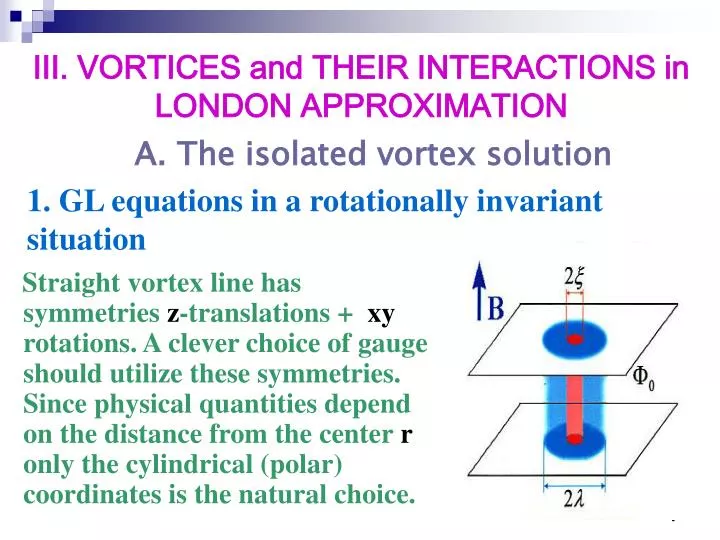
1. GL equations in a rotationally invariant situation

1. 1. GL equations in a rotationally invariant situation III. VORTICES and THEIR INTERACTIONS in LONDON APPROXIMATION A. The isolated vortex solution Straight vortex line has symmetries z-translations + xy rotations. A clever choice of gauge should utilize these symmetries. Since physical quantities depend on the distance from the center r only the cylindrical (polar) coordinates is the natural choice.

2. azimuthal vector field tangential vector field Using polar coordinates one chooses the following Ansatz (which includes a choice of the “unitary” gauge):

3. Details: polar coordinates The vector potential Partial derivatives

4. Magnetic field B is indeed a function of r only

5. Supercurrent Current therefore flows around the vortex.

6. GL equations Supercurrent equation has the azimuthal component only Similarly the nonlinear Schroedinger equation takes a form This should be supplemented by a set of four boundary conditions at the center and far away.

7. 2. Boundary condition and asymptotics near the vortex core. Near the center one expects a maximum of magnetic field B(0) leading to linear potential: Asymptotics of the order parameter at is assumed to be a power

8. Substituting this single vortex Ansatz into the NLSE one obtains: Leading terms are two: The order parameter therefore vanishes at the center of the vortex core as r for a single fluxon vortex. Nearr=0, we can use an expansion inr.

9. 3. Boundary conditions outside the core. Numerical solution Far away flux quantization gives The order parameter therefore exponentially approaches its bulk value in SC Using the four boundary conditions and linearity of both A and f at origin one can effectively use the “shooting” method to find the vortex solution

10. Exercise 2: transform the GL equations for a single vortex into a dimensionless form and solve it numerically using the shooting method fork=1, 10. A good simple fit for order parameter allris available: A simple expression for the magnetic field distribution can be obtained in phenomenologically important case of strongly type II superconductors using the London approximation

11. 4. The London electrodynamics outside vortex cores. Magnetic field of a vortex for Far enough from the vortex cores one generally makes the London appr. (even for many vortices) Covariant derivative

12. Supercurrent and Londons’ eqs In this case the supercurrent equation takes a London form: Taking 2D curl of the Maxwell equation

13. one obtains for a single vortex phase field: This is transformed into Londons’ equations in the presence of a straight vortex:

14. Field of a single vortex The eqs. are mathematically identical to the those for the Green’s function of the Klein-Gordon eqs and therefore can be solved by Fourier transform.

15. which has a pole. Inverse Fourier transform therefore will fall off exponentially: where is the Hankel function

16. The core cutoff Exponential tail Most of the flux for k>>1 passes through the x<r<l region. The core region fraction is insignificant:

17. The supercurrent distribution Taking a derivative the supercurrent is calculated One observes a rather long range decrease of the supercurrent between the coherence length and the penetration depth distances.

18. 5. Vortex carrying multiple flux quanta Then in the Laplacian we will have to replace and asymptotics at r=0 changes to: Core is much larger. As a result these vortices have larger energy and are difficult to find.

19. E. The line energy and interaction between vortices 1. Line Energy for The vortex line energy densitye is defined as the Gibbs energy of vortex solution minus . Neglecting the core and the condensation energy, we have:

20. In the London limit ( ) cov. gradient is proportional to supercurrent: This replaces the Maxwell energy. Integration by parts gives

21. Using the Londons equation One sees that the bulk integral vanishes and the inner boundary gives To calculate the derivative one uses magnetic field in the intermediate region

22. Consistency check: contribution of the core to energy is indeed small for k>>1, but just logarithmically

23. 2. Interaction between two straight vortices Consider two parallel straight vortices The London equation is linear in magnetic field. Therefore within range of its validity

24. The interaction line energy (potential) between two straight vortices is defined by Neglecting cores and using the trickofintegration by part as before one obtains from the London equation with two sources

25. To estimate the multiple internal boundary contribution, we first approximate the derivatives Since we will always (while using Londons appr.) assume r>>x the last term which is Powerwise small in 1/kwill be dropped

26. The two solitons energy is therefore proportional to magnetic field The interaction energy is

27. Force per unit length: Parallel vortices repel, anti-parallel attract, however the picture is more complicated than that: the force between curved vortices is of the vector-vector type

28. 3. Vortices as line - like objects Curved Abrikosov vortices in London approximation are infinitely thin elastic lines with interaction energy Brandt, JLTP (1991) Interaction is therefore mainly magnetic, hence pair - wise (superposition principle).

29. 4. Lorentz force of a current on the fluxon. Magnetic field affects current (moving charges) via the Lorentz force Current consequently applies a force in the opposite direction on fluxon due to Newton’s 3rd law.

30. F0 J FL FL JV In particular, force of vortex at on vortex at can be written as: The same logic leads to repultion between a vortex and an antivortex pointing to a vector – vector type of interaction Ao, Thoules, PRL 70, 2159 (93)

31. 5. Flux flow and dissipation. The Lorentz force on vortices which causes their motion is balanced in the stationary flow state by the friction force due to gapless excitations in the vortex cores. The vortex mass is negligible. Phenomenologically the friction force is described (in 2D) by:

32. The overdamped dynamics results in motion of vortices with a constant velocity across the boundary of length L. It produces the flux change Leading, using Maxwell eqs., to the voltage

33. which in turn implies a finite flux flow Ohmic resistivity Unless some other force like pinning obstructs the motion, the SC loses its second “defining” property: zero conductivity

34. The phenomenological Bardeen – Stephen model Let us assume that the dissipation which happens mainly in the normal cores is the same as in normal metal with resistivity . The fraction of area covered by the cores is proportional to B: The resistivity therefore is the same fraction of the normal state resistivity

35. How fast vortices can move? When the magnetic field reaches the cores cover the whole area and one is supposed to recover the whole normal state conductivity. This fixes the coefficient. Now the friction constant can be estimated: We will return to this later using the time dependent GL eqs. Within the Bardeen – Stephen model the vortex velocity is

36. For the Nb films One gets velocities of 20m/sec and 600m/sec for the critical and the depaitring current values of J respectively

37. For YBCO film One gets velocities of 20m/sec and 200km/sec. Boltz et al (2003)

38. 6. Simulation of vortex arrays Given all the forces one can simulate the vortex system using Runge – Kutta … When random disorder or thermal fluctuations are important they are introduces via random potential or force respectively (the Langeven method). The problem becomes that of mechanics of points or lines. Here the gaussian (usually white noice) Langeven random force represents thermal fluctuations

39. Pinning force is assumed to be well represented by a gaussian random pinning potential with certain correlator: Fangohr et al (2001)

40. Some sample results in 2D The I-V curves at different temperatures. Critical current Dynamical phase diagram in 2D Koshelev (1994)

41. Structure functions and hexatic order Fangohr et al (2001) Hellerquist et al (1996)

42. Summary 1. An isolated Abrikosov vortex carries in most cases one unit of magnetic flux. It has a normal core of radius x andthe SC magnetic “envelope” of the size lcarrying a vortex of supercurrent. 2. It has a small inertial mass and the creation energy (chemical potential) e 3. Parallel vortices repel each others, while curved ones interact via direction dependent vector force. 4. Interact with electric current in the mixed state. The current might induce the flux flow with finite resistance.

43. Details: Singular functions The polar angle function at the origin x=y=0 and has a “mild” singularity- a cut at y=0. For singular functions generally In particular To prove this let us take integral over arbitrary circle.

44. for function Using derivatives formula in polar coordinates one finds that the line integral is: This is true for any