Download
1 / 37
380 likes | 507 Views
Verifying cloud and boundary-layer forecasts. Robin Hogan Ewan O’Connor, Natalie Harvey, Thorwald Stein, Anthony Illingworth, Julien Delanoe, Helen Dacre, Helene Garcon University of Reading, UK Chris Ferro, Ian Jolliffe, David Stephenson University of Exeter, UK. How skillful is a forecast?.

E N D
Verifying cloud and boundary-layer forecasts Robin Hogan Ewan O’Connor, Natalie Harvey, Thorwald Stein, Anthony Illingworth, Julien Delanoe, Helen Dacre, Helene Garcon University of Reading, UK Chris Ferro, Ian Jolliffe, David Stephenson University of Exeter, UK
How skillful is a forecast? ECMWF 500-hPa geopotential anomaly correlation • Most model evaluations of clouds test the cloud climatology • What about individual forecasts? • Standard measure shows ECMWF forecast “half-life” of ~6 days in 1980 and ~9 days in 2000 • But virtually insensitive to clouds!
Geopotential height anomaly Vertical velocity • Cloud has smaller-scale variations than geopotential height because it is separated by around two orders of differentiation: • Cloud ~ vertical wind ~ relative vorticity ~ 2streamfunction ~ 2pressure • Suggests cloud observations would be a more stringent test of models
Overview • Desirable properties of verification measures (skill scores) • Usefulness for rare events • Equitability: is the “Equitable Threat Score” equitable? • Testing the skill of cloud forecasts from seven models • What is the “half life” of a cloud forecast? • Testing the skill of cloud forecasts from space • Which cloud types are best forecast and which types worst? • Testing the skill of boundary-layer type forecasts • New diagnosis from Doppler lidar
Cloud fraction Chilbolton Observations Met Office Mesoscale Model ECMWF Global Model Meteo-France ARPEGE Model KNMI RACMO Model Swedish RCA model
Raw (1 hr) resolution 1 year from Murgtal DWD COSMO model Joint PDFs of cloud fraction b a d c • 6-hr averaging …or use a simple contingency table
Contingency tables Model cloud Model clear-sky Observed cloud Observed clear-sky For given set of observed events, only 2 degrees of freedom in all possible forecasts (e.g. a & b), because 2 quantities fixed: - Number of events that occurred n =a +b +c +d - Base rate (observed frequency of occurrence) p =(a +c)/n
Desirable properties of verification measures • “Equitable”: all random forecasts receive expected score zero • Constant forecasts of occurrence or non-occurrence also score zero • Difficult to “hedge” • Some measures reward under- or over-prediction • Useful for rare events • Almost all widely used measures are “degenerate” in that they asymptote to 0 or 1 for vanishingly rare events • “Linear”: so that can fit an inverse exponential for half-life • Useful for overwhelmingly common events… • Base-rate independent… • Bounded… For a full discussion see Hogan and Mason, Chapter 3 of Forecast Verification 2nd edition:
Skill versus cloud-fraction threshold • Consider 7 models evaluated over 3 European sites in 2003-2004 • Two equitable measures: Heidke Skill Score and Log of Odds Ratio HSS LOR • LOR implies skill increases for larger cloud-fraction threshold • HSS implies skill decreases significantly for larger cloud-fraction threshold
Extreme dependency scores • Stephenson et al. (2008) explained this behavior: • Almost all scores have a meaningless limit as “base rate” p 0 • HSS tends to zero and LOR tends to infinity • Solved with their Extreme Dependency Score: • Problem: inequitable and easy to hedge: just forecast clouds all the time • Hogan et al. (2009) proposed the symmetric version SEDS: • Ferro and Stephenson (2011) proposed Symmetric Extremal Dependence Index • where hit rate H = a/(a+c) and false alarm rate F = b/(b+d) • Robust for rare and overwhelmingly common events
Skill versus cloud-fraction threshold SEDS HSS LOR • SEDS has much flatter behaviour for all models (except for Met Office which underestimates high cloud occurrence significantly)
Skill versus height • Verification using SEDS reveals: • Skill tends to slowly decrease at tropopause • Mid-level clouds (4-5 km) most skilfully predicted, particularly by Met Office • Boundary-layer clouds least skilfully predicted
Asymptotic equitability For some measures, expected score for random forecast only tends to zero for a large number of samples: these are asymptotically equitable • “Equitable Threat Score” is slightly inequitable for n < 30 • Should call it Gilbert Skill Score • ORSS, EDS, SEDS & SEDI approach zero much more slowly with n • For events that occur 2% of the time need n > 25,000 before magnitude of expected score is less than 0.01 • Hogan et al. (2010) showed that inequitable measures can be scaled to make them equitable but tricky numerical operation • Alternatively be sure sample size is large enough and report CIs on verification measures
Forecast “half life” Met Office DWD 2007 2004 3.0 d • Fit an inverse-exponential: • S0 is the initial score and t1/2 is the half-life • Noticeably longer half-life fitted after 36 hours • Same thing found for Met Office rainfall forecast (Roberts 2008) • First timescale due to data assimilation and convective events • Second due to more predictable large-scale weather systems 2.7 days 2.6 days 3.2 d 3.1 days 2.9 days 4.0 days 2.7 days 3.1 d 2.9 days 2.4 days 4.3 days 2.9 days 4.3 days 2.7 days
A-train verification: July 2006 GSS and LOR misleading: skill increases or decreases with cloud fraction SEDS and SEDI much more robust Both models underestimate mid- and low-level clouds (partly a snow issue at ECMWF) Highest skill: winter upper-troposphere mid-latitudes Lowest skill: tropical and sub-tropical boundary-layer clouds Tropical deep convection somewhere in between!
How is the boundary layer modelled? • Met Office model has explicit boundary-layer types (Lock et al. 2000)
Doppler-lidar retrieval of BL type Most probable boundary-layer type II: Stratocu over stable surface layer IIIb: Stratocumulus-topped mixed layer Ib: Stratus Usually the most probable type has a probability greater than 0.9 Now apply to two years of data and evaluate the type in the Met Office model Harvey, Hogan and Dacre (2012)
Forecast skill random
Forecast skill: stability b a c d random • Surface layer stable? • Model very skilful (but basically predicting day versus night) • Better than persistence (predicting yesterday’s observations)
Forecast skill: cumulus a b c d random • Cumulus present (given the surface layer is unstable)? • Much less skilful than in predicting stability • Significantly better than persistence
Forecast skill: decoupled b a d c random • Decoupled (as opposed to well-mixed)? • Not significantly more skilful than a persistence forecast
Forecast skill:multiple cloud layers? b a d c random • Cumulus under statocumulus as opposed to cumulus alone? • Not significantly more skilful than a random forecast • Much poorer than cloud occurrence skill (SEDI 0.5-0.7)
Take-home messages • Pressure is too easy to forecast; verify with clouds instead! • Half life of cloud forecasts is 2.5-4 days rather than 9-10 days • ETS is not strictly equitable: call it Gilbert Skill Score instead • But GSS and most others are misleading for rare events • I recommend the Symmetric Extremal Dependence Index • Global verifications shows mid-lat winter ice clouds have most skill, tropical boundary-layer clouds have no skill at all! • Relevant publications • Cloud-forecast half-life: Hogan, O’Connor & Illingworth (QJ 2009) • Asymptotic equitability: Hogan, Ferro, Jolliffe & Stephenson (WAF 2010) • SEDI: Ferro and Stephenson (WAF 2011) • Comparison of verification measures and calculation of confidence intervals: Hogan and Mason (2nd Ed of “Forecast Verification” 2011) • Doppler-lidar BL type: Harvey, Hogan & Dacre (Submitted to QJRMS) • Global verification: Hogan, Stein, Garcon & Delanoe (ERL in prep)
Cloud fraction in 7 models • All models except DWD underestimate mid-level cloud • Some have separate “radiatively inactive” snow (ECMWF, DWD); Met Office has combined ice and snow but still underestimates cloud fraction • Wide range of low cloud amounts in models • Not enough overcast boxes, particularly in Met Office model • Mean & PDF for 2004 for Chilbolton, Paris and Cabauw 0-7 km Illingworth et al. (BAMS 2007)
Skill-Bias diagrams Reality (n=16, p=1/4) Forecast Under-prediction No bias Over-prediction Best possible forecast - Positive skill Random forecast Negative skill Random unbiased forecast Constant forecast of occurrence Constant forecast of non-occurrence Worst possible forecast Hogan and Mason (2011)
Hedging“Issuing a forecast that differs from your true belief in order to improve your score” (e.g. Jolliffe 2008) • Hit rate H=a/(a+c) • Fraction of events correctly forecast • Easily hedged by randomly changing some forecasts of non-occurrence to occurrence H=0.5 H=0.75 H=1
Some reportedly equitable measures HSS = [x-E(x)] / [n-E(x)]; x = a+d ETS = [a-E(a)] / [a+b+c-E(a)] E(a) = (a+b)(a+c)/nis the expected value of a for an unbiased random forecasting system Simple attempts to hedge will fail for all these measures LOR = ln[ad/bc] ORSS = [ad/bc – 1] / [ad/bc + 1] Random and constant forecasts all score zero, so these measures are all equitable, right?
Extreme dependency score • Stephenson et al. (2008) explained this behavior: • Almost all scores have a meaningless limit as “base rate” p 0 • HSS tends to zero and LOR tends to infinity • They proposed the Extreme Dependency Score: • where n = a + b + c + d • It can be shown that this score tends to a meaningful limit: • Rewrite in terms of hit rate H =a/(a +c) and base rate p =(a +c)/n : • Then assume a power-law dependence of H on p as p 0: • In the limit p 0 we find • This is useful because random forecasts have Hit rate converging to zero at the same rate as base rate: d=1 so EDS=0 • Perfect forecasts have constant Hit rate with base rate: d=0 so EDS=1
Extreme dependence scores Extreme Dependence Score • Stephenson et al. (2008) • Inequitable • Easy to hedge Symmetric EDS • Hogan et al. (2009) • Asymptotically equitable • Difficult to hedge Symmetric Extremal Dependence Index • Ferro and Stephenson (2011) • Base-rate independent • Robust for both rare and overwhelmingly common events
Expected values of a–d for a random forecasting system may score zero: S[E(a), E(b), E(c), E(d)] = 0 But expected score may not be zero! E[S(a,b,c,d)] = S P(a,b,c,d)S(a,b,c,d) Width of random probability distribution decreases for larger sample size n A measure is only equitable if positive and negative scores cancel Which measures are equitable? ETS & ORSS are asymmetric n = 16 n = 80
Possible solutions • Ensure n is large enough that E(a) > 10 • Inequitable scores can be scaled to make them equitable: • This opens the way to a new class of non-linear equitable measures Report confidence intervals and “p-values” (the probability of a score being achieved by chance)
Key properties for estimating ½ life • We wish to model the score S versus forecast lead time t as: • where t1/2 is forecast “half-life” • We need linearity • Some measures “saturate” at high skill end (e.g. Yule’s Q / ORSS) • Leads to misleadingly long half-life • ...and equitability • The formula above assumes that score tends to zero for very long forecasts, which will only occur if the measure is equitable
Why is half-life less for clouds than pressure? • Different spatial scales? Convection? • Average temporally before calculating skill scores: • Absolute score and half-life increase with number of hours averaged
Forecast skill: Nocturnal stratocu b a d c random • Stratocumulus present (given a stable surface layer)? • Marginally more skilful than a persistence forecast • Much poorer than cloud occurrence skill (SEDI 0.5-0.7)