Download
1 / 1
10 likes | 168 Views
A high-resolution global ocean model of ROMS and its application to GRACE. Ocean Model

E N D
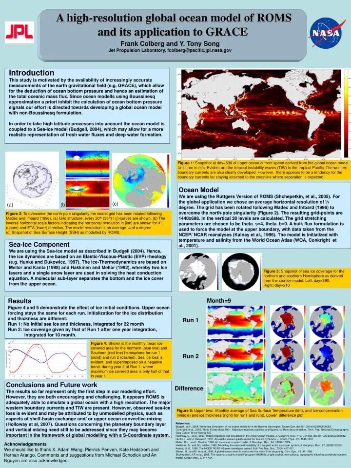
A high-resolution global ocean model of ROMS and its application to GRACE Ocean Model We are using the Ruttgers Version of ROMS (Shchepetkin, et al., 2005). For the global application we chose an average horizontal resolution of ¼ degree. The grid has been rotated following Madec and Imbard (1996) to overcome the north-pole singularity (Figure 2). The resulting grid-points are 1440x698. In the vertical 30 levels are calculated. The grid stretching parameters are chosen to be theta_s=4, theta_b=0. A bulk flux formulation is used to force the model at the upper boundary, with data taken from the NCEP/ NCAR reanalyses (Kalnay et al., 1996). The model is initialized with temperature and salinity from the World Ocean Atlas (WOA, Conkright et al., 2001). • Sea-Ice Component • We are using the Sea-Ice model as described in Budgell (2004). Hence, the ice dynamics are based on an Elastic-Viscous-Plastic (EVP) rheology (e.g. Hunke and Dukowicz, 1997). The Ice-Thermodynamics are based on Mellor and Kanta (1998) and Hakkinen and Mellor (1992), whereby two Ice layers and a single snow layer are used in solving the heat conduction equation. A molecular sub-layer separates the bottom and the ice cover from the upper ocean. Run 1 Run 2 Difference Figure 5: Upper two: Monthly average of Sea Surface Temperature (left), and Ice-concentration (middle) and ice thickness (right) for run1 and run2. Lower difference plot. Conclusions and Future work The results so far represent only the first step in our modelling effort. However, they are both encouraging and challenging. It appears ROMS is adequately able to simulate a global ocean with a high resolution. The major western boundary currents and TIW are present. However, observed sea-ice loss is evident and may be attributed to by unmodelled physics, such as aspects of shelf-basin exchange and/ or upper ocean convective mixing (Holloway et al, 2007). Questions concerning the planetary boundary layer and vertical mixing need still to be addressed since they may become important in the framework of global modelling with a S-Coordinate system. Frank Colberg and Y. Tony Song Jet Propulsion Laboratory, fcolberg@pacific.jpl.nasa.gov Introduction This study is motivated by the availability of increasingly accurate measurements of the earth gravitational field (e.g. GRACE), which allow for the deduction of ocean bottom pressure and hence an estimation of the total oceanic mass flux. Since ocean modells using Boussinesq approximation a priori inhibit the calculation of ocean bottom pressure signals our effort is directed towards developing a global ocean model with non-Boussinesq formulation. In order to take high latitude processes into account the ocean model is coupled to a Sea-Ice model (Budgell, 2004), which may allow for a more realistic representation of fresh water fluxes and deep water formation. Figure 1: Snapshot at day=630 of upper ocean current speed derived from the global ocean model. Units are in m/s. Evident are the tropical instability waves (TIW) in the tropical Pacific. The western boundary currents are also clearly developed. However, there appears to be a tendency for the boundary currents for staying attached to the coastline where separation is expected.. (c) (a) (b) Figure 2: To overcome the north-pole singularity the model grid has been rotated following Madec and Imbard (1996). (a) Grid structure: every 20th (35th) I (j)-curves are shown. (b) The inverse horizontal scale factors indicating the horizontal resolution in [km] are shown for XI, (upper) and ETA (lower) direction. The model resolution is on average ¼ of a degree. (c) Snapshot of Sea Surface Height (SSH) as modelled by ROMS. Figure 3: Snapshot of sea ice coverage for the northern and southern Hemisphere as derived from the sea-ice model. Left: day=390, Right: day=210 Results Figure 4 and 5 demonstrate the effect of ice initial conditions. Upper ocean forcing stays the same for each run. Initialization for the ice distribution and thickness are different: Run 1: No initial sea ice and thickness, Integrated for 22 month Run 2: Ice coverage given by that of Run 1 after one year integration, Integrated for 10 month. Month=9 Figure 4: Shown is the monthly mean ice covered area for the northern (blue line) and Southern (red line) hemisphere for run 1 (solid) and run 2 (dashed). Sea ice loss is evident, and superimposed on a negative trend, during year 2 of Run 1, where maximum ice covered area is only half of that in year 1. References Budgell, W.P., 2004, Numerical Simulation of ice-ocean variability in the Barents Sea region, Ocean Dyn.,doi:10.1007/s1023600500083. Conkright, et al., 2002, World Ocean Atlas 2001: Objective analyses statistics and figures, cd-Rom documentation, Tech. Rep. National Oceanographic Data Center, Silver Spring, MD. Holloway, G., et al., 2007, Water properties and circulation in the Arctic Ocean models, J. Geophys. Res., 112, C04S03, doi:10.1029/2006JC003642. Hunke E. and J. Dukuwicz, 1997, An elastic-viscous-plastic model for sea ice dynamics, J. Comp. Phys., 27, 1849-1867. Mellor, G.L., and L. Kantha, 1989, An ice-ocean coupled model. J. Geophys. Res., 94, 10937-10954. Hakkinen, S., and G.L. Mellor, 1992, Modelling the seasonal variability of a coupled arctic ice-ocean system, J. Geophys. Res., 97, 20285-20303. Kalnay, et al., 1996, The NCEP/ NCAR 40-year reanalyses project, Bull. Am. Met. Soc., 77(3), 437-471. Madec, G., and M. Imbard, 1996, A global ocean mesh to overcome the North Pole singularity, Clim. Dyn., 12, 381-388. Shchepetkin, A.F. et al., 2005, The regional oceanic modelling system (ROMS): a split-explicit, free-surface, topography-following-coordinate oceanic model, Ocean Mod., 9, 347-404. Acknowledgements We should like to thank X. Adam Wang, Pierrick Penven, Kate Hedstrom and Hernan Arango. Comments and suggestions from Michael Schodlok and An Nguyen are also acknowledged.