Results

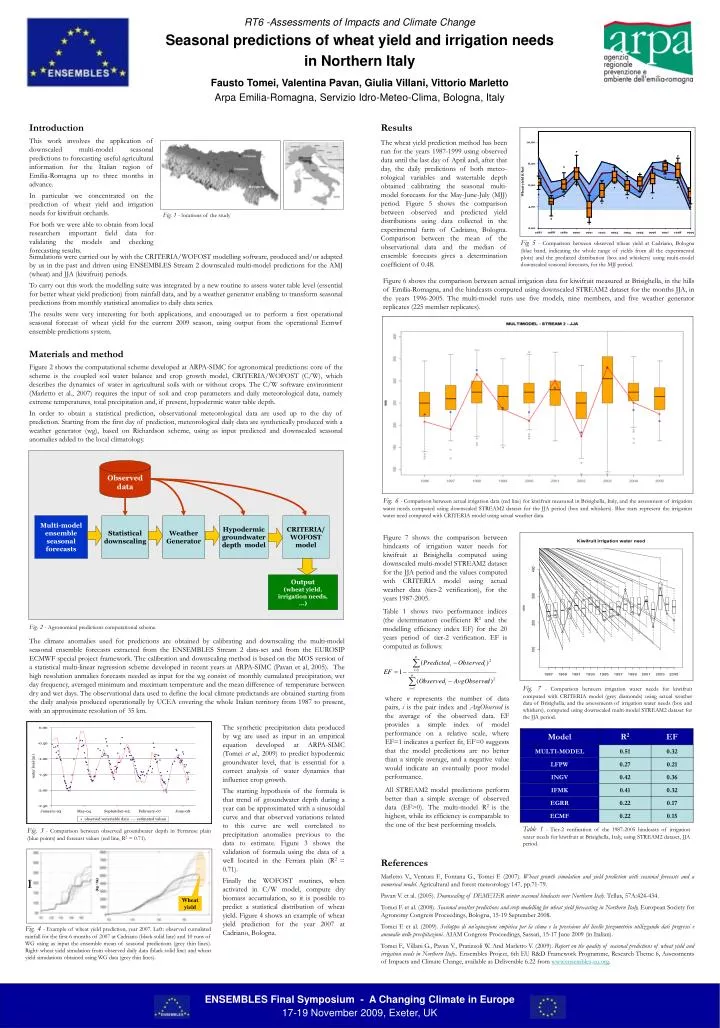
1. Brisighella Observed data Multi-model ensemble seasonal forecasts Statistical downscaling Weather Generator Hypodermic groundwater depth model CRITERIA/ WOFOST model Output (wheat yield, irrigation needs, …) Fig. 2 - Agronomical predictions computational scheme. Wheat yield Introduction This work involves the application of downscaled multi-model seasonal predictions to forecasting useful agricultural information for the Italian region of Emilia-Romagna up to three months in advance. In particular we concentrated on the prediction of wheat yield and irrigation needs for kiwifruit orchards. For both we were able to obtain from local researchers important field data for validating the models and checking forecasting results. Results The wheat yield prediction method has been run for the years 1987-1999 using observed data until the last day of April and, after that day, the daily predictions of both meteo-rological variables and watertable depth obtained calibrating the seasonal multi-model forecasts for the May-June-July (MJJ) period. Figure 5 shows the comparison between observed and predicted yield distributions using data collected in the experimental farm of Cadriano, Bologna. Comparison between the mean of the observational data and the median of ensemble forecasts gives a determination coefficient of 0.48. RT6 -Assessments of Impacts and Climate ChangeSeasonal predictions of wheat yield and irrigation needs in Northern ItalyFausto Tomei, Valentina Pavan, Giulia Villani, Vittorio MarlettoArpa Emilia-Romagna, Servizio Idro-Meteo-Clima, Bologna, Italy Fig. 1 - locations of the study Fig 5- Comparison between observed wheat yield at Cadriano, Bologna (blue band, indicating the whole range of yields from all the experimental plots) and the predicted distribution (box and whiskers) using multi-model downscaled seasonal forecasts, for the MJJ period. Simulations were carried out by with the CRITERIA/WOFOST modelling software, produced and/or adapted by us in the past and driven using ENSEMBLES Stream 2 downscaled multi-model predictions for the AMJ (wheat) and JJA (kiwifruit) periods. To carry out this work the modelling suite was integrated by a new routine to assess water table level (essential for better wheat yield prediction) from rainfall data, and by a weather generator enabling to transform seasonal predictions from monthly statistical anomalies to daily data series. The results were very interesting for both applications, and encouraged us to perform a first operational seasonal forecast of wheat yield for the current 2009 season, using output from the operational Ecmwf ensemble predictions system. Materials and method Figure 2 shows the computational scheme developed at ARPA-SIMC for agronomical predictions: core of the scheme is the coupled soil water balance and crop growth model, CRITERIA/WOFOST (C/W), which describes the dynamics of water in agricultural soils with or without crops. The C/W software environment (Marletto et al., 2007) requires the input of soil and crop parameters and daily meteorological data, namely extreme temperatures, total precipitation and, if present, hypodermic water table depth. In order to obtain a statistical prediction, observational meteorological data are used up to the day of prediction. Starting from the first day of prediction, meteorological daily data are synthetically produced with a weather generator (wg), based on Richardson scheme, using as input predicted and downscaled seasonal anomalies added to the local climatology. Figure 6 shows the comparison between actual irrigation data for kiwifruit measured at Brisighella, in the hills of Emilia-Romagna, and the hindcasts computed using downscaled STREAM2 dataset for the months JJA, in the years 1996-2005. The multi-model runs use five models, nine members, and five weather generator replicates (225 member replicates). Fig. 6- Comparison between actual irrigation data (red line) for kiwifruit measured in Brisighella, Italy, and the assessment of irrigation water needs computed using downscaled STREAM2 dataset for the JJA period (box and whiskers). Blue stars represent the irrigation water need computed with CRITERIA model using actual weather data. Figure 7 shows the comparison between hindcasts of irrigation water needs for kiwifruit at Brisighella computed using downscaled multi-model STREAM2 dataset for the JJA period and the values computed with CRITERIA model using actual weather data (tier-2 verification), for the years 1987-2005. Table 1 shows two performance indices (the determination coefficient R2 and the modelling efficiency index EF) for the 20 years period of tier-2 verification. EF is computed as follows: The climate anomalies used for predictions are obtained by calibrating and downscaling the multi-model seasonal ensemble forecasts extracted from the ENSEMBLES Stream 2 data-set and from the EUROSIP ECMWF special project framework. The calibration and downscaling method is based on the MOS version of a statistical multi-linear regression scheme developed in recent years at ARPA-SIMC (Pavan et al, 2005). The high resolution anmalies forecasts needed as input for the wg consist of monthly cumulated precipitation, wet day frequency, averaged minimum and maximum temperature and the mean difference of temperature between dry and wet days. The observational data used to define the local climate predictands are obtained starting from the daily analysis produced operationally by UCEA covering the whole Italian territory from 1987 to present, with an approximate resolution of 35 km. Fig. 7- Comparison between irrigation water needs for kiwifruit computed with CRITERIA model (grey diamonds) using actual weather data of Brisighella, and the assessments of irrigation water needs (box and whiskers), computed using downscaled multi-model STREAM2 dataset for the JJA period. where n represents the number of data pairs, i is the pair index and AvgObserved is the average of the observed data. EF provides a simple index of model performance on a relative scale, where EF=1 indicates a perfect fit, EF=0 suggests that the model predictions are no better than a simple average, and a negative value would indicate an eventually poor model performance. All STREAM2 model predictions perform better than a simple average of observed data (EF>0). The multi-model R2 is the highest, while its efficiency is comparable to the one of the best performing models. The synthetic precipitation data produced by wg are used as input in an empirical equation developed at ARPA-SIMC (Tomei et al., 2009) to predict hypodermic groundwater level, that is essential for a correct analysis of water dynamics that influence crop growth. The starting hypothesis of the formula is that trend of groundwater depth during a year can be approximated with a sinusoidal curve and that observed variations related to this curve are well correlated to precipitation anomalies previous to the data to estimate. Figure 3 shows the validation of formula using the data of a well located in the Ferrara plain (R2 = 0.71). Finally the WOFOST routines, when activated in C/W model, compute dry biomass accumulation, so it is possible to predict a statistical distribution of wheat yield. Figure 4 shows an example of wheat yield prediction for the year 2007 at Cadriano, Bologna. Table 1- Tier-2 verification of the 1987-2005 hindcasts of irrigation water needs for kiwifruit at Brisighella, Italy, using STREAM2 dataset, JJA period. Fig. 3- Comparison between observed groundwater depth in Ferrarese plain (blue points) and forecast values (red line, R2 = 0.71). References Marletto V., Ventura F., Fontana G., Tomei F. (2007).Wheat growth simulation and yield prediction with seasonal forecasts and a numerical model. Agricultural and forest meteorology 147, pp.71-79. Pavan V. et al. (2005). Downscaling of DEMETER winter seasonal hindcasts over Northern Italy. Tellus, 57A:424-434. Tomei F. et al. (2008). Seasonal weather predictions and crop modelling for wheat yield forecasting in Northern Italy, European Society for Agronomy Congress Proceedings, Bologna, 15-19 September 2008. Tomei F. et al. (2009). Sviluppo di un’equazione empirica per la stima e la previsione del livello piezometrico utilizzando dati pregressi e anomalie nelle precipitazioni. AIAM Congress Proceedings, Sassari, 15-17 June 2009 (in Italian). Tomei F., Villani G., Pavan V., Pratizzoli W. And Marletto V. (2009). Report on the quality of seasonal predictions of wheat yield and irrigation needs in Northern Italy.. Ensembles Project, 6th EU R&D Framework Programme, Research Theme 6, Assessments of Impacts and Climate Change, available as Deliverable 6.22 from www.ensembles-eu.org. Fig. 4- Example of wheat yield prediction, year 2007. Left: observed cumulated rainfall for the first 6 months of 2007 at Cadriano (black solid line) and 10 runs of WG using as input the ensemble mean of seasonal predictions (grey thin lines). Right: wheat yield simulation from observed daily data (black solid line) and wheat yield simulations obtained using WG data (grey thin lines). ENSEMBLES Final Symposium - A Changing Climate in Europe 17-19 November 2009, Exeter, UK