Reversals of the Geomagnetic Field

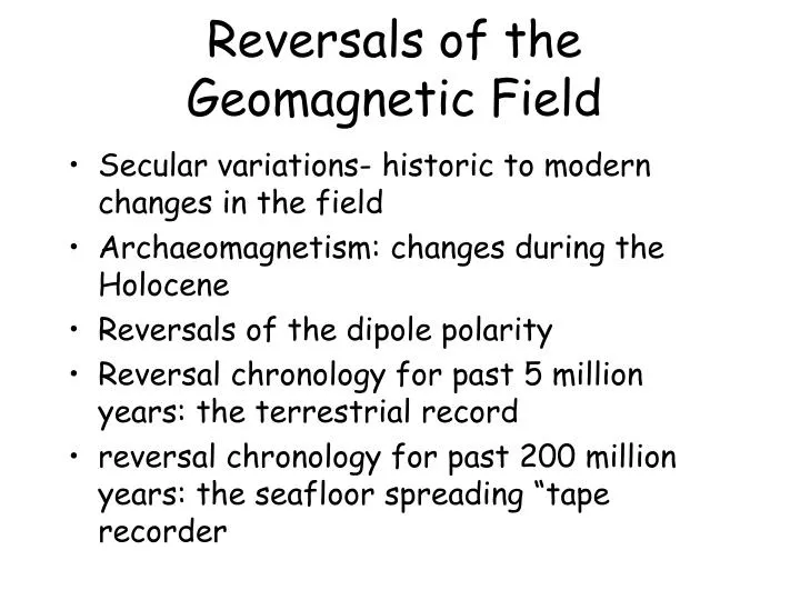
1. Reversals of the Geomagnetic Field Secular variations- historic to modern changes in the field Archaeomagnetism: changes during the Holocene Reversals of the dipole polarity Reversal chronology for past 5 million years: the terrestrial record reversal chronology for past 200 million years: the seafloor spreading “tape recorder

2. Locations of the north pole of the dipole component of the geomagnetic field from 1945-2000.

3. -30 to 800 BP 800 to 1940 BP 1940 to 3690 BP The north magnetic pole during the past 3700 years. -30 to 3690 BP Average pole position for all data (94 poles): 88.4 N 23.8 W 1.6 degrees from geographic North Pole Calibrated radiocarbon years before present, (B.P, AD1950=0)

4. units: nT/yr contour interval: 5 nT/yr Main field: 30,000 to 60,000 nT

5. units: minutes/yr contour interval: 2 min/yr

6. units: minutes/yr contour interval: 1 min/yr

7. Dipole moment determined from the strength of magnetization of archaeological material (archaeomagnetic results from TRM in ancient hearths and pottery) Years before present (BP)

8. Schematic plot of magnetic field variations in time dipole component non-dipole component

9. A snapshot of the 3D magnetic field structure simulated with the Glatzmaier-Roberts geodynamo model. Magnetic field lines are blue where the field is directed inward and yellow where directed outward. The rotation axis of the model Earth is vertical and through the center. A transition occurs at the core-mantle boundary from the intense, complicated field structure in the fluid core, where the field is generated, to the smooth, potential field structure outside the core. The field lines are drawn out to two Earth radii. Magnetic field is wrapped around the "tangent cylinder" due to the shear of the zonal fluid flow.

10. 500yrs after 500yrs before middle of reversal About “36,000 years” into the simulation the magnetic field underwent a reversal of its dipole moment (Figure 3), over a period of a little more than a thousand years. The intensity of the magnetic dipole moment decreased by about a factor of ten during the reversal and recovered immediately after, similar to what is seen in the Earth's paleomagnetic reversal record. Our solution shows how convection in the fluid outer core is continually trying to reverse the field but that the solid inner core inhibits magnetic reversals because the field in the inner core can only change on the much longer time scale of diffusion [2]. Only once in many attempts is a reversal successful, which is probably the reason why the times between reversals of the Earth's field are long and randomly distributed.

11. The key to determining the chronology of the geomagnetic field reversals is to be able to date the time during which robust magnetizations were attained in a given rock sample. The classical work was done in the latter half of the last century on basaltic rocks, which cool rapidly and acquire a strong thermo-remanent magnetization (TRM). These rocks can be dated effectively with the Potassium-Argon method, which uses the decay of K-40 into the chemically inert Ar-40. Ar-40 is trapped and accumulates in the rock only since the last time the rock was melted – the time when the basalt was extruded and solidified. While liquid, the prior Ar-40, a gas, leaves the magma. Since the basalt is extruded on the surface, cooling is rapid and the acquisition of TRM occurs soon after the trap is set for accumulation of Ar-40.

12. Reversal captured in Columbia River basalt flows ( Steens Mtn., Oregon: Miocene, 15.5 Ma)

13. Steens Mtn: Kiger Gorge from the Steens Mountain Loop Road

14. Steens Mtn: View northwest from the short trail/road to the summit.

15. High resolution record of geomagnetic field reversal 3500 yrs 3600 yrs Reversal captured in Columbia River basalt flows ( Steens Mtn., Oregon: Miocene, 15.5 Ma) Extrusions at rate of about 43 m/1000 yrs 5000 yrs Mankinen, et al., 1985, J. Geophys. Res., v. 90, p, 10400

16. Steens Mtn results: VGP’s in time

17. Magnetizations (DRM) recovered from deep ocean sediments

18. Magnetizations (DRM) recovered from deep ocean sediments Note minimum intensities during reversals

19. Geomagnetic field reversal chronology for past 5 million years based mainly on K-Ar dating of terrestrial volcanic rocks Why only to 5 Ma?

20. Geomagnetic field reversal chronology for past 5 million years based mainly on K-Ar dating of terrestrial volcanic rocks Why only to 5 Ma? Errors in K-Ar dates become too large compared to reversal periods

21. The chronology of geomagnetic field reversals earlier than 5 Ma is well preserved in the magnetization of basalts extruded on the ocean floor in the process of sea-floor spreading.

23. moho crust upper mantle lithosphere Seafloor spreading model Schematic representation of upper crustal magnetized layer Age, Ma 1200 deg C convecting mantle

24. moho crust upper mantle Seafloor spreading is a tape recorder of the geomagnetic field! The reversal chronology recorded on land Age, Ma The “tape drive” The recording head of the “tape recorder”

25. Marine magnetic anomalies • Ships tow magnetometers which measure the “total intensity” of the geomagnetic field, the magnitude of the geomagnetic field vector, often symbolized by F, or Fobs, to denote that it is the observed total intensity.These measurements lead to a plot of Fobs versus distance along the track.

26. Smoothly varying global field plus small, short wavelength effects due to crustal magnetizations magnetic field intensity,Fobs 0 distance along ship track

27. Marine Magnetic anomalies • Ships tow magnetometers which measure the “total intensity” of the geomagnetic field, the magnitude of the geomagnetic field vector, often symbolized by F, or Fobs , to denote that it is the observed total intensity. These measurements lead to a plot of Fobs versus distance along the track. • The main internal geomagnetic field (produced in the outer core), Fg, is determined for the earth as a function of time as the International Geomagnetic Reference Field (IGRF). • The IGRF field can then be subtracted from the observed value to produce a total intensity anomaly, DF= Fobs - Fg • DF results only from effects of rocks magnetized near the surface, and can thus be compared with models of the magnetization of the ocean bottom rocks.

28. Smoothly varying global field plus small, short wavelength effects of crustal magnitizations magnetic field intensity,Fobs 0 distance along ship track Total intensity anomaly, DF intensiy anomaly, DF 0 distance along ship track

29. Marine Magnetic anomalies The rocks with the strongest magnetizations by far are the basalts extruded and rapidly cooled, acquiring thermo-remanent magnetization (TRM) via the process of seafloor spreading.

30. Magnetic field lines for vertically downwards magnetization in cross-sectional view - - - - - - - - - - - - - - - - J + + + + + + + + + + + + + + +

31. Magnetic field lines for vertically upwards magnetization + + + + + + + + + + + + + + + J - - - - - - - - - - - - - - - -

32. Vertically downwards magnetization parallel to vertical earth’s field Earth’s field, He Magnetic field due to magnetized prism taken along the surface above the prism (directions only) ocean surface - - - - - - - - - - - - - - - - J + + + + + + + + + + + + + + +

33. Magnetized prism field adds to Earth’s field, DF positive Earth’s field, He Magnetic field due to magnetized prism taken along the surface above the prism (directions only) - - - - - - - - - - - - - - - - J + + + + + + + + + + + + + + +

34. Magnetized prism field perpendicular to He, DF = 0 Earth’s field, He Magnetic field due to magnetized prism taken along the surface above the prism (directions only) - - - - - - - - - - - - - - - - J + + + + + + + + + + + + + + +

35. Magnetized prism field subtracts from He, DF negative Earth’s field, He Magnetic field due to magnetized prism taken along the surface above the prism (directions only) - - - - - - - - - - - - - - - - J + + + + + + + + + + + + + + +

36. + Intensity anomaly, DF distance along track - sea surface axis of seafloor spreading Direction of modern geomagnetic field reversal reversal reversal reversal ocean bottom Basalt magnetized upon solidification along axis of spreading ridge

37. Intensity anomaly, DF distance along track Magnetization increases main field Magnetization decreases main field Magnetization decreases main field sea surface axis of seafloor spreading Direction of modern geomagnetic field reversal reversal reversal reversal ocean bottom Basalt magnetized upon solidification along axis of spreading ridge

38. Global bathymetry, showing ocean ridge system

39. Global bathymetry, showing ocean ridge system Mid-Atlantic Ridge East Pacific Rise

40. Global bathymetry, showing ocean ridge system Mid-Atlantic Ridge East Pacific Rise Map shown in next slide

41. Ship tracks across the East Pacific Rise which obtained the magnetic anomalies shown in the next slide. The measurements were made in the 1960’s by the Columbia University research vessel Eltanin. 21 20 19

42. Eltanin profiles of magnetic anomalies The vertical scale for total intensity anomaly, DF, is shown in “gammas”. This is the same as nanoTeslas or nT. The horizontal linesare at zero anomaly; the scale is thus minus 500 to plus 500 nT. Magnetic anomaly, gamma Ocean depth, km

43. The incredible symmetry of the Eltanin 19 profile ESE WNW WNW ESE total intensity anomaly calculated from model mirror image of measured profile to show symmetry measured profile of total intensity anomalies

44. Eltanin profiles of magnetic anomalies The four profiles show total intensity anomalies and bathymetry (ocean depth in km) along the four tracks shown on the previous map. Note that track 20 crosses the ridge system twice.

45. Also note that peaks and troughs in the curves can be correlated from track to track, indicating that the magnetized material on the ocean floor with a positive or negative magnetization can be traced along the strike of the ocean ridge system. These correlations are shown by the numbers, which identify correlatable features in the wiggly lines.

46. Modeling the magnetic anomaly pattern mirror image of measured profile to show symmetry ESE WNW Observed profile of total intensity anomalies WNW ESE total intensity anomaly calculated from model cross section through model of normal (black) and reversed (white) magnetized upper crust reversal chronology from paleomagnetic studies on land

47. moho crust upper mantle lithosphere Seafloor spreading model Schematic representation of upper crustal magnetized layer Age, Ma 1200 deg C convecting mantle

48. The seafloor spreading tape recorder extends the record of geomagnetic field reversals out as far as we have ocean basins- this turns out to be about 200 million years worth of recording.

49. All that is needed is to determine the timing of the recording system back beyond 5 million years.

50. How? Drilling to the bottom of the sediments that cover the basalts The Ocean Drilling Program, which started in 1968, and is still working, did just this throughout the world’s oceans.