Download
1 / 17
170 likes | 275 Views
Composite Interval Mapping Program. - Type of Study. - Genetic Design. Composite Interval Mapping Program. - Data and Options. Cumulative Marker Distance (cM). Map Function. QTL Searching Step. cM. Parameters Here for Simulation Study Only. Composite Interval Mapping Program. - Data.

E N D
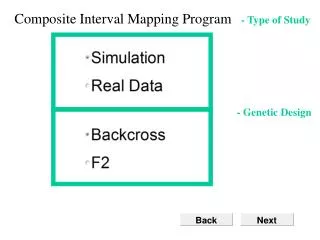
CompositeInterval Mapping Program - Type of Study - Genetic Design
CompositeInterval Mapping Program - Data and Options Cumulative Marker Distance (cM) Map Function QTL Searching Step cM Parameters Here for Simulation Study Only
CompositeInterval Mapping Program - Data Put Markers and Trait Data into box below OR
CompositeInterval Mapping Program - Analyze Data For CIM, Controlled Background Markers by Within cM Or Markers
CompositeInterval Mapping Program - Profile
CompositeInterval Mapping Program - Permutation Test #Tests Cut Off Point at Level Is Based on Tests.
r=a+b-2ab M a Q b N F2 Population – Three Point
Composite model for interval mapping and regression analysis zi: QTL genotype xik: marker genotype yi = + a* zi + km-2bkxik + ei Expected means: Qq: + a* + kbkxik = a* + XiB qq: + kbkxik = XiB Xi = (1, xi1, xi2, …, xi(m-2))1x(m-1) B = (, b1, b2, …, bm-2)T M1 x1 M1m1 1 +b1 m1m1 0
zi – conditional probability of Qq given markers of individual i and QTL position xik – coding for ‘effect’ of k-th marker of i Backcross: xik =1 if k-th marker of i is Mm =0 or –1 if k-th marker of i is mm km-2 – summation over all markers except two markers of current interval We want estimate a* and test if abs(a*) is big enough to claim that there is a QTL at the given location in an interval. The estimate B is not very important
Likelihood based CIM L(y,M|) = i=1n[1|if1(yi) + 0|if0(yi)] log L(y,M|) = i=1n log[1|if1(yi) + 0|if0(yi)] f1(yi) = 1/[(2)½]exp[-½(y-1)2], 1= a*+XiB f0(yi) = 1/[(2)½]exp[-½(y-0)2], 0= XiB Define 1|i= 1|if1(yi)/[1|if1(yi) + 0|if0(yi)] (1) 0|i= 0|if1(yi)/[1|if1(yi) + 0|if0(yi)] (2)
a* = i=1n1|i(yi-a*-XiB)/ i=1n1|i (3) = 1 (Y-XB)´/c B = (X´X)-1X´(Y-1a*) (4) 2 = 1/n (Y-XB)´(Y-XB) – a*2 c (5) • = (i=1n21|i +i=1n30|i)/(n2+n3) (6) Y = {yi}nx1, = {1|i}nx1, c = i=1n1|i
Hypothesis test H0: a*=0 vs H1: a*0 L0 = i=1nf(yi) B = (X´X)-1X´Y, 2=1/n(Y-XB)´(Y-XB) L1= i=1n[1|if1(yi) + 0|if0(yi)] LR = -2(lnL0 – lnL1) LOD = -(logL0 – logL1)
Likelihood based CIM for BC and F2 L(y,M|) = i=1n k=1g [k|ifk(yi)] log L(y,M|) = i=1n log[k=1gk|ifk(yi)] g=2 for BC, 3 for F2 fk(yi) = 1/[(2)½]exp[-½(y-k)2], k= gk+XiB k=1,…,g
Define k|i= k|if1(yi)/[k=1gk|if1(yi)] (1) B = k=1gk(X´X)-1X´(Y- gk) (2) gk = i=1nk|i(yi-XiB)/ i=1nk|i (3) 2 = 1/n i=1n k=1gk|i(yi-XiB - gk )2 (4) Y = {yi}nx1, k= {k|i}nx1