Download
1 / 25
250 likes | 260 Views
Utah State University GIS in Water Resources CEE 6440 Term Project. Hatim Geli. Building a VBA Toolbox to Perform the TOPMODEL. Fall 2007. http://techalive.mtu.edu/meec/module01/images/Watershed.jpg. Introduction.

E N D
Utah State University GIS in Water Resources CEE 6440Term Project Hatim Geli Building a VBA Toolbox to Perform the TOPMODEL Fall 2007 http://techalive.mtu.edu/meec/module01/images/Watershed.jpg
Introduction • One of the most important decision making tools in the field of water resources management is the hydrological model. • Required in some fields such as • Hydropower generation, • Irrigation Development, • Flood Control, • Early Warning, and • Drinking Water Supply.
Objectives • Use the Visual Basic for Application VBA within ArcGIS to build a toolbox • The purpose is to help in applying the semi-distributed model “TOPMODEL”.
TOPMODEL cont… The TOPMODEL is a semi-distributed physically based rainfall-runoff model developed by Beven and Kirkby (1979). It requires digitized elevation data, rainfall data, and potential evapotranspiration data and it predicts the resulting runoff and spatial soil water saturation pattern Figure 1: Topographic index and recharge rate.
Data and Basemap • Compute the Flow Direction grid Fdr, • Compute the Flow Accumulation grid Fac, • Compute the Stream Definition grid, in which the stream is defined by a threshold area of 33,000 km2 in this study decrease the amount of time of computation required, • Create the Stream Segmentation, • Create the Catchment Grid, • Catchment polygon feature class, • Create the Adjoint Catchments polygon feature class, • Create Batch Point feature class which contains the point feature class for the USGS steam gage flow measurements, • Create the Watershed polygon feature class which include all the subcatchments upstream the stream gage, • Finally extract the Blue River Basin grid based on the Batch Point and the Watershed polygon.
Data and Basemap cont… 1233 km2 , by the USGS Figure 2: Basemap for Blue River Basin
The modeling steps • Assumption and estimation values for f, T0, , ,and K0 • Calculate lambda and gamma, • Assume or estimate initial baseflow , at time step t=1, • Calculate the mean water table depth , at t=1, • Calculate the local time table depth at location i , at time step t=1, • Calculate Qv, at time step t=1, • Using the previous time step values and Equation 4 to calculate at t=2, • Calculate Qb from resulted in step 7, • Repeat steps 5 to 8 until t = T ,the total time length, • Evaluate each of the estimated zi to obtain the runoff generated at the outlet point.
Get the Toolbar Figure 3: Customize the Toolbar
Model Toolbox components Figure 4: Main Menu of the TOPMODEL Figure 5: Drop Down menu for the DEM Processing
Model Toolbar components cont… Figure 7: Topographic Index calculation menu Figure 6: Slope calculation menu
Model Toolbar components cont… Figure 8: Main Run menu Figure 9: Output menu
Sample model run cont… Figure 10: Sample run for the “Slope” menu
Sample model run cont… Figure 11: Sample run for the “Slope” menu cont…
Sample model run cont… Figure 12: Sample run for the “Topo. Index” menu cont…
Sample model run cont… Figure 13: Sample run for the “Topo. Index” menu cont…
Sample model run cont… Figure 14: Map showing the DEM and the Topo. Index
Sample VBA Code of the “Run” button Private Sub cmdRun_Click() . Tsat = CDbl(txtTsat.Text) pRasModel.Script = " [out1]= [atanb] / " & Tsat . Set pOutRaster3 = pRasMathOp.Ln(pOutRaster1) Gamma = pRasterStats.Mean MsgBox "Your gamma is =" & pRasterStats.Mean & vbLf + vbLf + _ "Now your model will continue...“ For I = 1 To N – 1 qbase(I) = Exp(-Gamma) * Exp(-Fscale * Zbar(I)) pRasModel5.Script = " [out4]= " & Zbar(I) & " - [flnsa]" pRasModel5.Script = "[out5]=" & -Fscale & " * [out4] “ pRasModel5.Script = "[out6]= " & Ksat * alpha & " * [out5] “ Set Zi(I) = pRasModel5.BoundRaster("out4") If Precip(I) = 0 Then Runoff(I) = 0 + qbase(I) * Area * 1000000 * 35.3147 Else Runoff(I) = (EvaZi(Zi(I), Precip(I), DTheta, pWS) * 35.3147) / 3600 / 24 + qbase(I) * Area * 1000000 * 35.3147 End If Zbar(I + 1) = Zbar(I) + DTheta * (qbase(I) - qvert(I)) Next I Private Function EvaZi pRasModel.Script = " [out1]= ([Zi] < 0) > 0 “ … 'pRasModel.Script = " [out1]= ([Zi] > 0 and [Zi] < " & pRain / 100 / DTheta & ") > 0 “… End Function Figure 15: Sample VBA code for the model “Run” button
Sample model run cont… Figure 16: The “Run” menu
Sample model run cont… Figure 17: The Output menu
Sample model run cont… Figure 18: Plot of mean water table
Sample model run cont… Figure 19: Plot Actual and Predicted Streamflow
Future • Increase the model capabilities to allow working with distributed soil parameters. • Also to allow working with distributed rainfall as well as snow. • Include evapotranspiration component, • Include component to allow working with real-time data,
Get help for VBA codes for ESRI ArcGIS functions • ESRI Developer Network • http://edn.esri.com/ • ArcGIS Desktop Help • http://webhelp.esri.com/arcgisdesktop/9.2/index.cfm?TopicName=welcome