Download
1 / 24
320 likes | 966 Views
III. Gabor Transform . III-A Definition. Standard form:. Alternative definitions:. normalization. Main Reference S. Qian and D. Chen, Sections 3-2 ~ 3-6 in Joint Time-Frequency Analysis: Methods and Applications , Prentice-Hall, 1996. Other References

E N D
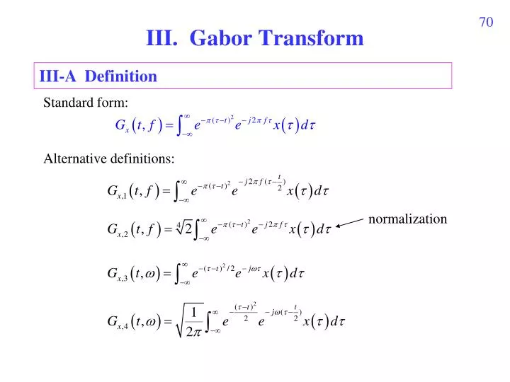
III. Gabor Transform III-A Definition Standard form: Alternative definitions: normalization
Main Reference • S. Qian and D. Chen, Sections 3-2 ~ 3-6 in Joint Time-Frequency Analysis: Methods and Applications, Prentice-Hall, 1996. • Other References • D. Gabor, “Theory of communication”, J. Inst. Elec. Eng., vol. 93, pp. 429-457, Nov. 1946. (最早提出 Gabor transform) • M. J. Bastiaans, “Gabor’s expansion of a signal into Gaussian elementary signals,” Proc. IEEE, vol. 68, pp. 594-598, 1980. • R. L. Allen and D. W. Mills, Signal Analysis: Time, Frequency, Scale, and Structure, Wiley- Interscience. • S. C. Pei and J. J. Ding, “Relations between Gabor transforms and fractional Fourier transforms and their applications for signal processing,” IEEE Trans. Signal Processing, vol. 55, no. 10, pp. 4839-4850, Oct. 2007.
註: 許多文獻把 Gabor transform 直接就稱作 Short-time Fourier transform (STFT),實際上, Gabor transform 是 STFT 當中的一個 special case.
III-B Approximation of the Gabor Transform Although the range of integration is from − to, due to the fact that when |a| > 1.9143 when |a| > 4.7985 the Gabor transform can be simplified as:
III-C Why Do We Choose the Gaussian Function as a Mask (1) Among all functions, the Gaussian function has the advantage that the area in time-frequency distribution is minimal. (和其他的 STFT 相比,比較能夠同時讓 time-domain 和 frequency domain 擁有較好的清晰度) w(t) 太寬 time domain 的解析度較差 W(f) = FT[w(t)]太寬 frequency domain 的解析度較差 (2) 由於 Gaussian function 是 FT 的 eigenfunction,因此 Gabor transform 在 time domain 和 frequency domain 的性質將互相對稱
Uncertainty Principle (Heisenberg, 1927) For a signal x(t), if when |t| , then σtσf 1/4π where ,
(Proof of Henseinberg’s uncertainty principle): From simplification, we consider the case where μt = μf = 0 Then, use Parseval’s theorem if X(f) = FT[x(t)]
From Schwarz’s inequality (using |a+b|2 + |a–b|2 2|a|2 )
For Gaussian function use use [工具書] M. R. Spiegel, Mathematical Handbook of Formulas and Tables, McGraw-Hill, 3rd Ed., 2009.
同理, 所以對 Gaussian function 而言, 滿足下限
Special relation between the Gaussian function and the rectangular function Gaussian function is also an eigenmode in optics, radar system, and other electromagnetic wave systems. (will be illustrated in the 7th week)
III-D Simulations Gabor transform forGaussian function exp(t2) rec-STFT, B = 0.5 forGaussian function exp(t2) f-axis f-axis t-axis t-axis
x(t) = cos(2 t) when t < 10, x(t) = cos(6 t) when 10 t < 20, x(t) = cos(4 t) when t 20
Gabor transform of s(t) Gabor transform of r(t) f-axis f-axis t-axis t-axis for –9 t 1, s(t) = 0 otherwise,
Gabor transform for s(t) + r(t) f-axis t-axis
III-E Properties of Gabor Transforms (1) Integration property When k 0, When k = 0, When k = 1, (recovery property) • (2) Shifting property • If y(t) = x(t – t0), then . • (3) Modulation property • If y(t) = x(t)exp(j2f0t), then
(4)Special inputs: (a) When x() = (), (b) When x() = 1, (symmetric for the time and frequency domains) (5) Linearity property If z() = x() + y() andGz(t, f ), Gx(t, f ) and Gy(t, f ) are their Gabor transforms, then Gx(t, f ) = Gx(t, f ) + Gy(t, f ) (6) Power integration property:
(7) Energy sum property Gx(t, f ) and Gy(t, f ) are the Gabor transforms of x() and y() (8) Power decayed property If x(t) = 0 for t > t0, then . i.e., for t > t0. If for f > f0, then for f > f0.
III-F Generalization of Gabor Transforms larger σ: higher resolution in the time domain lower resolution in the frequency domain smaller σ: higher resolution in the frequency domain lower resolution in the time domain
Gabor transform forGaussian function exp(t2) = 0.2 Gabor transform forGaussian function exp(t2) = 5 f-axis f-axis t-axis t-axis
處理對 time resolution 相對上比 frequency resolution 敏感的信號 • Using the generalized Gabor transform with larger σ • Using other time unit instead of second 例如,原本 t (單位:sec) f (單位: Hz) 對聲音信號可以改成 t (單位: 0.1 sec) f (單位:10 Hz)
附錄三:Matlab 寫程式的原則 (1) 迴圈能避免就儘量避免 (2) 儘可能使用 Matrix 及 Vector operation (3) 能夠不在迴圈內做的運算,則移到迴圈外 (4) 寫一部分即測試,不要全部寫完再測試 (縮小範圍比較容易 debug) (5) 先測試簡單的例子,成功後再測試複雜的例子 註:作業 Matlab Program (or C program) 鼓勵各位同學儘量用精簡的 方式寫。Program 越精簡,或執行速度越快,分數就越高。 問答題鼓勵各位同學寫得越完整越好
一些重要的 Matlab 指令 (1) function: 放在第一行,可以將整個程式函式化 (2) tic, toc: 計算時間 tic 為開始計時,toc 為顯示時間 (3) find: 找尋一個 vector 當中不等於 0 的entry 的位置 範例:find([1 0 0 1]) = [1, 4] find(abs([-5:5])<=2) = [4, 5, 6, 7, 8] (因為 abs([-5:5])<=2 = [0 0 0 1 1 1 1 1 0 0 0]) (4) : Hermitian (transpose + conjugation),. : transpose (5) imread: 讀圖, image, imshow, imagesc: 將圖顯示出來, (註: 較老的 Matlab 版本 imread 要和 double 並用 A=double(imread(‘Lena.bmp’)); (6) imwrite: 製做圖檔
(7) xlsread: 由 Excel 檔讀取資料 (8) xlswrite: 將資料寫成 Excel 檔 (9) aviread: 讀取 video 檔 (10) dlmread: 讀取 *.txt 或其他類型檔案的資料 (11) dlmwrite: 將資料寫成 *.txt 或其他類型檔案