Download
1 / 8
90 likes | 228 Views
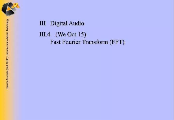
III Digital Audio III.4 (We Oct 15) Fast Fourier Transform (FFT). Recall these facts: The representation. w r = w(rΔ) = w(r/N) = ∑ m = 0, 1, 2, 3, ... N-1 c m e i2 . m r/N.

E N D
III Digital Audio III.4 (We Oct 15) Fast Fourier Transform (FFT)
Recall these facts: The representation wr = w(rΔ) = w(r/N) = ∑m = 0, 1, 2, 3, ... N-1 cm e i2.mr/N identifies the sequence w = (w0,w1,w2,…,wN-1) as a vector in the N-dimensional complex space ¬N. So our samples of fundamental frequency f = 1 are identified with the vectors w ∈ ¬N. We have a scalar product — similar to the highschool formula (u,v) = |u|.|v|.cos(u,v): v u Have N exponential functions e0, e1, e2,... eN-1 that are represented as vectors in ¬N em = (em(r) = ei2.mr/N)r = 0,1,2,...N-1 〈em, em〉 = 1, 〈em, ek〉 = 0 m ≠ k = orthogonality relationsmentioned above! The e0, e1, e2,... eN-1 = orthonormal basis like for normal 3 space! (ortho ~ perpendicular, normal ~ length 1) They replace the sinusoidal functions! ek 90o 90o 90o el em
And this: Every sound sample vector w = (w0,w1,w2,…,wN-1) in ¬N can be written as a linear combination w = ∑m = 0, 1, 2, 3, ... N-1 cmem of the exponential functions, and the (uniquely determined) coefficients cm are calculated via cm = 〈w, em〉 = 1/N.∑r = 0, 1, 2, 3, ... N-1 wr e-i2.mr/N ek So we have to calculate the coefficients cm!The big question is:How fast can we do this? N can be very large!!Think of CD: 44100 samples/second 90o 90o 90o el em
The Fast Fourier Transform is an algorithm for a faster calculation of the coefficients cm = 〈w, em〉 = 1/N.∑r = 0, 1, 2, 3, ... N-1 wr e-i2.mr/N It was published 1965 in a 5-page (!) paper in Math. Comput.19: 297–301 entitled An Algorithm for the Machine Calculation of Complex Fourier Series by James W. Cooley (IMB T.J. Watson Research Center) and John W. Tuckey (Princeton University and AT&T Bell Labs). This is one of the most cited papers. The algorithm was used already 1805 by the great mathematician Carl Friedrich Gauss for astronomical calculations, but not recognized since his text was written in Latin… Let us now see how much faster the FFT algorithm is. And faster than what? John W. Tuckey Carl F. Gauss
For the calculation of the N values cm = 〈w, em〉 = 1/N.∑r = 0, 1, 2, 3, ... N-1 wr e-i2.mr/N we suppose that the values wr for all r = 0,1,... N-1 E(N) = e-i2/N are all known. We have to calculate the powers e-i2.2/N = E(N)2,... e-i2.(N-1)/N = E(N)N-1 by N-2 multiplications. And then for all m, r the N2 multiplications wr × e-i2.mr/N And we have to add N-1 times the products and make one division by N per m, adding up to N2 additional operations. This all adds up to 2N2 + N-2 operations, which grows in a quadratic manner with respect to N. Example: N = 44100: 2N2 + N-2 = 3 889 664 098 ≈ 3.889 Billions
The FFT algorithm allows instead of 2N2 + N-2 operations, which grows in a quadratic manner with respect to N. a growth of only N.log(N), which means a much lesser growth ans shown here for the quotient (2N2 + N-2)/N.log(N) Compared to 3.889 × 10⁹, we only get 2.048 × 10⁵ here!
The FFT algorithm supposes that N is a power of 2, N = 2M, not only an even number as before. We then have this fundamental fact when stepping to the double 2N of the sample size: Fourier(2N) ≤ 2.Fourier(N) + 8N where Fourier(N) means the growth function of N, we leave this as an intuitive concept for our needs, ok? Then the FFT growth formula Fourier(N) ≤ N.log(N) can be proved without efforts inductively (supposing N is large!), i.e. for 2N if we suppose it true for N: Fourier(2N) ≤ 2.Fourier(N) + 8N ≤ 2N.log(N) + 8N ≤ 2N(log(N) +8) ≤ 2N.log(2N) So we are left with the proof of the above fundamental fact!
And this is the trick: The sound sample vector w = (w0,w1,w2,…,w2N-1) in ¬2N is split into two parts of length N each: w = (w0,w1,w2,…,w2N-1) ¬2N odd even w− = (w1, w3,…,w2N-1) w+ = (w0, w2, w4,…,w2N-2) ¬N Fourier(N) Fourier(N) c+ = (c+0, c+1, c+2,…,c+N-1) c− = (c−0, c−1,…, c−N-1) Have this decisive formula: cr = (c+r + e(N)r . c−r)/2, i.e. per r we have 2 multiplications, one addition and a total of 2N powers of e(N). Together with the 2.Fourier(N) operations for the c+ and c− we have Fourier(2N) ≤ 3 × 2N + 2N + 2.Fourier(N) = 2.Fourier(N) + 8N, QED.