Digital image processing Chapter 3. Image sampling and quantization

1. Digital image processing Chapter 3. Image sampling and quantization IMAGE SAMPLING AND IMAGE QUANTIZATION 1. Introduction 2. Sampling in the two-dimensional space Basics on image sampling The concept of spatial frequencies Images of limited bandwidth Two-dimensional sampling Image reconstruction from its samples The Nyquist rate. The alias effect and spectral replicas superposition The sampling theorem in the two-dimensional case Non-rectangular sampling grids and interlaced sampling The optimal sampling Practical limitations in sampling and reconstruction 3. Image quantization 4. The optimal quantizer The uniform quantizer 5. Visual quantization Contrast quantization Pseudo-random noise quantization Halftone image generation Color image quantization

2. Digital image processing Chapter 3. Image sampling and quantization 1.Introduction Fig 1 Image sampling and quantization / Analog image display

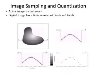
3. f(x,y) x y Digital image processing Chapter 3. Image sampling and quantization 2.Sampling in the two-dimensional space Basics on image sampling

4. Digital image processing Chapter 3. Image sampling and quantization The concept of spatial frequencies - Grey scale images can be seen as a 2-D generalization of time-varying signals (both in the analog and in the digital case); the following equivalence applies:

5. Digital image processing Chapter 3. Image sampling and quantization • Images of limited bandwidth • Limited bandwidth image = 2-D signal with finite spectral support: • F(νx, νy) = the Fourier transform of the image: The spectrum of a limited bandwidth image and its spectral support

6. Digital image processing Chapter 3. Image sampling and quantization Two-dimensional sampling (1) The common sampling grid = the uniformly spaced, rectangular grid: Image sampling = read from the original, spatially continuous, brightness functionf(x,y), only in the black dots positions ( only where the grid allows):

7. Digital image processing Chapter 3. Image sampling and quantization Two-dimensional sampling (2) • Question: How to choose the values Δx, Δy to achieve: • the representation of the digital image by the min. number of samples, • at (ideally) no loss of information? • (I. e.: for a perfectly uniform image, only 1 sample is enough to completely represent the image => sampling can be done with very large steps; on the opposite – if the brightness varies very sharply => very many samples needed) • The sampling intervals Δx, Δy needed to have no loss of information depend on the spatial frequency content of the image. • Sampling conditions for no information loss – derived by examining the spectrum of the image  by performing the Fourier analysis: • The sampling grid function g(Δx, Δy) is periodical with period (Δx, Δy) => can be expressed by its Fourier series expansion:

8. Digital image processing Chapter 3. Image sampling and quantization Two-dimensional sampling (3) • Since: • Therefore the Fourier transform of fS is:  Thespectrum of the sampled image = the collection of an infinite number of scaled spectral replicas of the spectrum of the original image, centered at multiples of spatial frequencies 1/Δx, 1/ Δy.

9. Digital image processing Chapter 3. Image sampling and quantization Original image spectrum – 3D Original image spectrum – 2D Original image 2-D rectangular sampling grid Sampled image spectrum – 3D Sampled image spectrum – 2D

10. Digital image processing Chapter 3. Image sampling and quantization Image reconstruction from its samples Let us assume that the filtering region R is rectangular, at the middle distance between two spectral replicas:

11. Digital image processing Chapter 3. Image sampling and quantization • Since the sinc function has infinite extent => it is impossible to implement in practice the ideal LPF • it is impossible to reconstruct in practice an image from its samples without error if we sample it at the Nyquist rates. Practical solution: sample the image at higher spatial frequencies + implement a real LPF (as close to the ideal as possible). 1-D sinc function 2-D sinc function

12. Digital image processing Chapter 3. Image sampling and quantization The Nyquist rate. The aliasing. The fold-over frequencies Note: Aliasing may also appear in the reconstruction process, due to the imperfections of the filter! How to avoid aliasing if cannot increase the sampling frequencies? By a LPF on the image applied prior to sampling! The Moire effect “Jagged” boundaries

13. Digital image processing Chapter 3. Image sampling and quantization Non-rectangular sampling grids. Interlaced sampling grids Interlaced sampling Optimal sampling = Karhunen-Loeve expansion:

14. Digital image processing Chapter 3. Image sampling and quantization Image reconstruction from its samples in the real case The question is: what to fill in the “interpolated” (new) dots? Several interpolation methods are available; ideally – sinc function in the spatial domain; in practice – simpler interpolation methods (i.e. approximations of LPFs).

15. Digital image processing Chapter 3. Image sampling and quantization Image interpolation filters:

16. Digital image processing Chapter 3. Image sampling and quantization Image interpolation examples: 1. Rectangular (zero-order) filter, or nearest neighbour filter, or box filter: Original Sampled Reconstructed

17. Digital image processing Chapter 3. Image sampling and quantization Image interpolation examples: 2. Triangular (first-order) filter, or bilinear filter, or tent filter: Original Sampled Reconstructed

18. Digital image processing Chapter 3. Image sampling and quantization Image interpolation examples: 3. Cubic interpolation filter, or bicubic filter – begins to better approximate the sinc function: Original Sampled Reconstructed

19. Digital image processing Chapter 3. Image sampling and quantization Practical limitations in image sampling and reconstruction Fig. 7 The block diagram of a real sampler & reconstruction (display) system Fig. 8 The real effect of the interpolation

20. Digital image processing Chapter 3. Image sampling and quantization 3. Image quantization Fig. 9 The quantizer’s transfer function 3.1. Overview

21. Digital image processing Chapter 3. Image sampling and quantization • 3.2. The uniform quantizer • The quantizer’s design: • Denote the input brightness range: • Let B – the number of bits of the quantizer => L=2B reconstruction levels • The expressions of the decision levels: • The expressions of the reconstruction levels: • Computation of the quantization error: for a given image of size M×N pixels, U– non-quantized, and U’ – quantized => we estimate the MSE: E.g. B=2 => L=4

22. Digital image processing Chapter 3. Image sampling and quantization Examples of uniform quantization and the resulting errors: B=1 => L=2 Non-quantized image Quantized image Quantization error; MSE=36.2 The histogram of the non-quantized image

23. Digital image processing Chapter 3. Image sampling and quantization Examples of uniform quantization and the resulting errors: B=2 => L=4 Non-quantized image Quantized image Quantization error; MSE=15 The histogram of the non-quantized image

24. Digital image processing Chapter 3. Image sampling and quantization Examples of uniform quantization and the resulting errors: B=3 => L=8; false contours present Non-quantized image Quantized image Quantization error; MSE=7.33 The histogram of the non-quantized image

25. Digital image processing Chapter 3. Image sampling and quantization 3.2. The optimal (MSE) quantizer (the Lloyd-Max quantizer)

26. Digital image processing Chapter 3. Image sampling and quantization (Gaussian) , or(Laplacian) (variance , - mean)

27. Digital image processing Chapter 3. Image sampling and quantization Examples of optimal quantization and the quantization error: B=1 => L=2 Non-quantized image Quantized image The quantization error; MSE=19.5 The evolution of MSE in the optimization, starting from the uniform quantizer The non-quantized image histogram

28. Digital image processing Chapter 3. Image sampling and quantization Examples of optimal quantization and the quantization error: B=2 => L=4 Non-quantized image Quantized image The quantization error; MSE=9.6 The evolution of MSE in the optimization, starting from the uniform quantizer The non-quantized image histogram

29. Digital image processing Chapter 3. Image sampling and quantization Examples of optimal quantization and the quantization error: B=3 => L=8 Non-quantized image Quantized image The quantization error; MSE=5 The evolution of MSE in the optimization, starting from the uniform quantizer The non-quantized image histogram

30. Digital image processing Chapter 3. Image sampling and quantization 3.3. The uniform quantizer = the optimal quantizer for the uniform grey level distribution:

31. Digital image processing Chapter 3. Image sampling and quantization 3.4. Visual quantization methods • In general – if B<6 (uniform quantization) or B<5 (optimal quantization) => the "contouring" effect (i.e. false contours) appears in the quantized image. • The false contours (“contouring”) = groups of neighbor pixels quantized to the same value <=> regions of constant gray levels; the boundaries of these regions are the false contours. • The false contours do not contribute significantly to the MSE, but are very disturbing for the human eye => it is important to reduce the visibility of the quantization error, not only the MSQE. • Solutions: visual quantization schemes, to hold quantization error below the level of visibility. • Two main schemes: (a) contrast quantization; (b) pseudo-random noise quantization Uniform quantization, B=4 Optimal quantization, B=4 Uniform quantization, B=6

32. Digital image processing Chapter 3. Image sampling and quantization 3.4. Visual quantization methods • a. Contrast quantization • The visual perception of the luminance is non-linear, but the visual perception of contrast is linear • uniform quantization of the contrast is better than uniform quantization of the brightness • contrast = ratio between the lightest and the darkest brightness in the spatial region • just noticeable changes in contrast: 2% => 50 quantization levels needed  6 bits needed with a uniform quantizer (or 4-5 bits needed with an optimal quantizer)

33. Digital image processing Chapter 3. Image sampling and quantization • Examples of contrast quantization: • For c=u1/3:

34. Digital image processing Chapter 3. Image sampling and quantization • Examples of contrast quantization: • For the log transform:

35. Digital image processing Chapter 3. Image sampling and quantization b. Pseudorandom noise quantization (“dither”) Large dither amplitude Uniform quantization, B=4 Prior to dither subtraction Small dither amplitude

36. Digital image processing Chapter 3. Image sampling and quantization

37. Digital image processing Chapter 3. Image sampling and quantization Halftone images generation Fig.14 Digital generation of halftone images Demo:http://markschulze.net/halftone/index.html Fig.15 Halftone matrices

38. Digital image processing Chapter 3. Image sampling and quantization Fig.3.16

39. Digital image processing Chapter 3. Image sampling and quantization Color images quantization Fig.17 Color images quantization