Download

1 / 39
570 likes | 1.06k Views
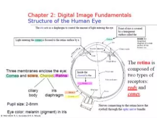
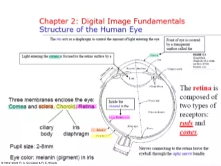
Image Processing Chapter 2 Digital Image Fundamentals. White Light. Colours Absorbed. Green Light. Reflected Light. The colours that we perceive are determined by the nature of the light reflected from an object

E N D
White Light Colours Absorbed Green Light Reflected Light • The colours that we perceive are determined by the nature of the light reflected from an object • For example, if white light is shone onto a green object most wavelengths are absorbed, while green light is reflected from the object
Simple Image Model • Monochrome(Gray) Image : f(x,y) • f(x,y) = intensity value at coordinates (x,y) • 0 < f(x,y) < ∞ ; f(x,y) is energy
Simple Image Model • Simple image formation • f(x,y) = i(x,y)r(x,y) • i(x,y): illumination (determined by ill. Source) • 0 < i(x,y) < ∞ • r(x,y) reflectance (determined by imaged object) • 0 < r(x,y) < 1 • In real situation • Lmin≤ l (=f(x,y)) ≤ Lmax • L : gray level
Sampling & Quantization • Image sampling • Digitization of spatial coordinates (x,y) • A digital sensor can only measure a limited number of samples at a discrete set of energy levels • Quantization • Amplitude digitization • In all types of sensors, quantization of the sensor output completes the process of generating digital image. • The quality of a digital image is determined to a large degree by the number of samples and discrete gray levels used in sampling and quantization
Sampling & Quantization Remember that a digital image is always only an approximation of a real world scene
Representing Digital Image • a digital image is composed of M rows and N columns of pixels each storing a value • Pixel values are most often grey levels in the range 0-255(black-white) • Images can easily be represented as matrices
Representing Digital Image Continuous image Digital Image The notation (0,1), is used to signify the the second sample along the first row, not the actual physical coordinates when the image was sampled
Storage • For M x N image with L(=2k) discrete gray level • The number, b, of bits required to store the image is b = MNk ex1) 1024 x 1024 x 8bit = 1Mbytes
What is Digital Image? • Digital image : x,y,f(x,y), three values are all discretized • Pixel : Image elements, Picture elements, Pels
What is Digital Image? • Comparison • f(x,y) : 2D still image • f(x,y,z) : 3D object • f(x,y,t) : Video or Image Sequence • f(x,y,z,t) : moving 3D object • Spatial Resolution (x,y) • Spatial resolution is the smallest discernible detail in an image • A line pair : a line and its adjacent space • A widely used definition of resolution is the smallest number of discernible line pairs per unit distance • ex) 100 line pairs/mm • But, unit distance or unit area is omitted in most cases
Spatial Resolution • The spatial resolution of an image is determined by how sampling was carried out • Spatial resolution simply refers to the smallest discernable detail in an image • Vision specialists will often talk about pixel size • Graphic designers will talk about dots per inch (DPI) 5.1 Megapixels
Gray-level Resolution • Gray-level resolution is the smallest discernible change in gray level (but, highly subjective!) • Due to hardware considerations, we only consider quantization level • Usually an integer power of 2. The most common level is 28=256 • However, we can find some systems that can digitize the gray levels of an image with 10 to 12 bits of accuracy.
Isopreference curves • Effects produced on image quality by varying N and K • Relation between subjective image quality and resolution • Tested by images with low/medium/high detail • Result • A few gray levels may be needed for high detailed image • Perceived quality in the other two image categories remained the same in some intervals in which the spatial resolution was increased, but the number of gray levels actually decrease
Aliasing • Shannon sampling theorem • if the function is sampled at a rate equal to or greater than twice its highest frequency, it is possible to recover completely the original function from its samples • if the function is undersampled, then a phenomenon called aliasing corrupts the sampled image • The corruption is in the form of additional frequency components being introduced into the sampled function. These are called aliased frequencies • Nyquist freq. = 0.5 x sampling rate
Aliasing • Except for a special case, it is impossible to satisfy the sampling theorem in practice • The principal approach for reducing the aliasing effects on an image is to reduce its high-frequency components by blurring the image prior to sampling • However, aliasing is always present in a sampled image • The effect of aliased frequencies can be seen under the right conditions in the form of so-called Moiré patterns
Zooming and Shrinking • Zooming : requires two steps • Creation of a new pixel location • Assignment of a gray level to those new locations • Nearest neighbour interpolation (ex 500 x 500 image) • Laying an imaginary 750 x 750 grid over the original image • Spacing in the grid will be less than one pixel • Look for the closest pixel in the original image and assign its gray level to the new pixel in the grid. • Fast but produces checkerboard effect that is particularly objectionable at high factor of magnification. • Pixel replacement • Applicable when we want to increase with integer number of times • We can duplicate each column • Then we duplicate each row of the enlarged image.
Zooming and Shrinking • Bilinear interpolation (four neighbours of point) • Let x`, y` a point in the zoomed image • v (x`, y`) a gray level assigned to it • v is given by • v (x`, y`) = ax` + by` + cx`y` +d • The coefficients are determined from the four equations using the four neighbours. • Shrinking is done in the same manner as just described for zooming
Neighbors of a Pixel • N4(p) : 4-neighbors of pixel p(x, y) • { p(x+1, y), p(x-1, y), p(x, y+1), p(x, y-1)} • ND(p) : diagonal neighbors of pixel p(x, y) • { p(x+1, y+1), p(x-1, y-1), p(x-1, y+1), p(x+1, y-1)} • N8(p) : 8-neighbors of pixel p(y,x) • N8(p) = N4(p) UND(p) • Some of the neighbors of pixel p lie outside the digital image if the pixel p is on the border of the image
Connectivity • Def: Two pixels are connected, if they are adjacent in some sense and if their gray levels are similar. • Let V be the set of gray levels used to define connectivity; e.g. V={1} for the connectivity of pixels with value 1 in a binary image with 0 and 1.
Connectivity (cont.) • In a gray-scale image, for the connectivity of pixels with a range of intensity values of , say, 100 to 120, it follows that V={100,101,102,…,120}. • We consider three types of connectivity: • 4-connectivity Two pixels p and q with values from V are 4-connected if q is in the set N4(p) .
Connectivity (cont.) • 8-connectivity • Two pixels p and q with values from V are 8-connected if q is in the set N8(p) .
Connectivity (cont.) • m-connectivity (mixed connectivity) • Two pixels p and q with values from V are m-connected if • (i) q is in N4(p) , or • (ii) q is in ND( p) and ND( p) ∩ N4 (q) is empty
Path • A (digital) path(or curve) from pixel p at (x,y) to pixel q at (s,t) is a sequence of distinct pixels with coordinates (x0,y0), (x1,y1), …,, (xn,yn) where (x0,y0) =(x,y), (xn,yn)=(s,t), and pixel (xi,yi) and (xi-1,yi-1) are adjacent for 1≤ i ≤ n • n is the length of the path • If (x0,y0) =(xn,yn), the path is a closed path • The path can be defined 4-,8-,m-paths depending on adjacency type
Connectivity • Let S be a subset of pixels in an image. Two pixels p and q are said to be connected in S if there exists a path between them consisting entirely of pixels in S • For any pixel p in S, the set of pixels that are connected to it in S is called a connected component of S. • If it only has one connected component, then set S is called a connected set. • Let R be a subset of pixels in an image. We call R a region of the image if R is a connected set • The boundary of a region R is the set of pixels in the region that have one or more neighbors that are not in R
Distance Measures • Let pixels be • p=p(x,y), q=q(s,t), z=z(u,v) • D() is a distance function or metric if (a) D(p,q) ≥ 0 (D(p,q)=0 iff p=q) (b) D(p,q) = D(q,p) (c) D(p,z) ≤ D(p,q) + D(q,z)
Distance Measures • Euclidean distance De(p,q) = [(x-s)2 + (y-t)2]1/2 • D4distance (city-block distance) D4(p,q) = |x-s| + |y-t| Distance from (x,y) less than or equal some value r from a diamond centered at (x,y) The pixels with D4 = 1 are the 4-neighbor 2 2 1 2 2 1 0 1 2 2 1 2 2
Distance Measures • D8 distance (chessboard distance) D8(p,q) = max(|x-s|, |y-t|) 2 2 2 2 2 2 1 1 1 2 2 1 0 1 2 2 1 1 1 2 2 2 2 2 2
Arithmetic/Logic Operations • Arithmetic operation • Addition: p+q • Subtraction: p-q • Multiplication: pxq • Division: p ÷ q • Logic Operation • AND: p AND q (p. q) • OR: p OR q (p + q) • COMPLEMENT: NOT q ( q )
Logic Operations • Try the following problems • 1, 5, 7, 9, 11, 13, 15