PART II THE MARKET SYSTEM

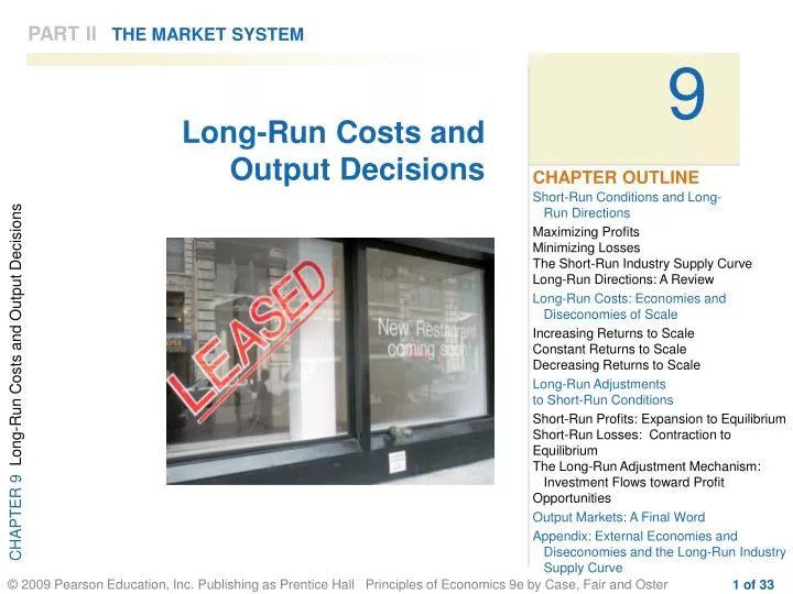
1. Long-Run Costs and Output Decisions PART IITHE MARKET SYSTEM 9 CHAPTER OUTLINE Short-Run Conditions and Long- Run Directions Maximizing ProfitsMinimizing LossesThe Short-Run Industry Supply CurveLong-Run Directions: A Review Long-Run Costs: Economies and Diseconomies of Scale Increasing Returns to ScaleConstant Returns to ScaleDecreasing Returns to Scale Long-Run Adjustmentsto Short-Run Conditions Short-Run Profits: Expansion to EquilibriumShort-Run Losses: Contraction to EquilibriumThe Long-Run Adjustment Mechanism: Investment Flows toward Profit Opportunities Output Markets: A Final Word Appendix: External Economies and Diseconomies and the Long-Run Industry Supply Curve

2. Long-Run Costs and Output Decisions • We begin our discussion of the long run by looking at firms in three short-run circumstances: • firms earning economic profits, • firms suffering economic losses but continuing to operate to reduce or minimize those losses, and • firms that decide to shut down and bear losses just equal to fixed costs. breaking even The situation in which a firm is earning exactly a normal rate of return.

3. Short-Run Conditions and Long-Run Directions Maximizing Profits Example: The Blue Velvet Car Wash

4. Short-Run Conditions and Long-Run Directions Maximizing Profits  FIGURE 9.1 Firm Earning Positive Profits in the Short Run A profit-maximizing perfectly competitive firm will produce up to the point where P* = MC. Profits are the difference between total revenue and total costs. At q* = 300, total revenue is $5 × 300 = $1,500, total cost is $4.20 × 300 = $1,260, and total profit = $1,500  $1,260 = $240.

5. Short-Run Conditions and Long-Run Directions Minimizing Losses operating profit (or loss) or net operating revenue Total revenue minus total variable cost (TR - TVC). ■ If revenues exceed variable costs, operating profit is positive and can be used to offset fixed costs and reduce losses, and it will pay the firm to keep operating. ■ If revenues are smaller than variable costs, the firm suffers operating losses that push total losses above fixed costs. In this case, the firm can minimize its losses by shutting down.

6. Short-Run Conditions and Long-Run Directions Minimizing Losses Producing at a Loss to Offset Fixed Costs: The Blue Velvet Revisited

7. Short-Run Conditions and Long-Run Directions Minimizing Losses  FIGURE 9.1 Firm Suffering Losses but Showing an Operating Profit in the Short Run When price is sufficient to cover average variable costs, firms suffering short-run losses will continue operating instead of shutting down. Total revenues (P* × q*) cover variable costs, leaving an operating profit of $90 to cover part of fixed costs and reduce losses to $135.

8. Short-Run Conditions and Long-Run Directions Minimizing Losses Shutting Down to Minimize Loss

9. Short-Run Conditions and Long-Run Directions Minimizing Losses  FIGURE 9.1 Firm Suffering Losses but Showing an Operating Profit in the Short Run At prices below average variable cost, it pays a firm to shut down rather than continue operating. Thus, the short-run supply curve of a competitive firm is the part of its marginal cost curve that lies above its average variable cost curve. shut-down point The lowest point on the average variable cost curve. When price falls below the minimum point on AVC, total revenue is insufficient to cover variable costs and the firm will shut down and bear losses equal to fixed costs.

10. Short-Run Conditions and Long-Run Directions The Short-Run Industry Supply Curve short-run industry supply curve The sum of the marginal cost curves (above AVC) of all the firms in an industry.  FIGURE 9.4 The Industry Supply Curve in the Short Run Is the Horizontal Sum of the Marginal Cost Curves (above AVC) of All the Firms in an Industry A profit-maximizing perfectly competitive firm will produce up to the point where P* = If there are only three firms in the industry, the industry supply curve is simply the sum of all the products supplied by the three firms at each price. For example, at $6, firm 1 supplies 100 units, firm 2 supplies 200 units, and firm 3 supplies 150 units, for a total industry supply of 450.

11. Short-Run Conditions and Long-Run Directions Long-Run Directions: A Review

12. Long-Run Costs: Economies and Diseconomies of Scale increasing returns to scale, or economies of scale An increase in a firm’s scale of production leads to lower costs per unit produced. constant returns to scale An increase in a firm’s scale of production has no effect on costs per unit produced. decreasing returns to scale, or diseconomies of scale An increase in a firm’s scale of production leads to higher costs per unit produced.

13. Long-Run Costs: Economies and Diseconomies of Scale Increasing Returns to Scale Example: Economies of Scale in Egg Production

14. Long-Run Costs: Economies and Diseconomies of Scale long-run average cost curve (LRAC) A graph that shows the different scales on which a firm can choose to operate in the long run.  FIGURE 9.5 A Firm Exhibiting Economies of Scale The long-run average cost curve of a firm shows the different scales on which the firm can choose to operate in the long run. Each scale of operation defines a different short run. Here we see a firm exhibiting economies of scale; moving from scale 1 to scale 3 reduces average cost.

15. Long-Run Costs: Economies and Diseconomies of Scale Constant Returns to Scale Technically, the term constant returns means that the quantitative relationship between input and output stays constant, or the same, when output is increased. Constant returns to scale mean that the firm’s long-run average cost curve remains flat.

16. Long-Run Costs: Economies and Diseconomies of Scale Decreasing Returns to Scale optimal scale of plantThe scale of plant that minimizes average cost.  FIGURE 9.6 A Firm Exhibiting Economies and Diseconomies of Scale Economies of scale push this firm’s average costs down to q*. Beyond q*, the firm experiences diseconomies of scale; q* is the level of production at lowest average cost, using optimal scale.

17. Long-Run Costs: Economies and Diseconomies of Scale Blood bank merger ‘good’ for Manatee Bradenton Herald.com “Northwest needed to be aligned with a larger organization to achieve economy of scale,” said J.B. Gaskins, Florida Blood Services vice president. “That economy of scale is good for the whole network, including Manatee County.”

18. Long-Run Adjustments to Short-Run Conditions Short-Run Profits: Expansion to Equilibrium  FIGURE 9.7 Firms Expand in the Long Run When Increasing Returns to Scale Are Available When economies of scale can be realized, firms have an incentive to expand. Thus, firms will be pushed by competition to produce at their optimal scales. Price will be driven to the minimum point on the LRAC curve.

19. Long-Run Adjustments to Short-Run Conditions Short-Run Profits: Expansion to Equilibrium In the long run, equilibrium price (P*) is equal to long-run average cost, short-run marginal cost, and short-run average cost. Profits are driven to zero: P* = SRMC = SRAC = LRAC Any price above P* means that there are profits to be made in the industry, and new firms will continue to enter. Any price below P* means that firms are suffering losses, and firms will exit the industry. Only at P* will profits be just equal to zero, and only at P* will the industry be in equilibrium.

20. Long-Run Adjustments to Short-Run Conditions Short-Run Losses: Contraction to Equilibrium  FIGURE 9.8 Long-Run Contraction and Exit in an Industry Suffering Short-Run Losses When firms in an industry suffer losses, there is an incentive for them to exit. As firms exit, the supply curve shifts from S0 to S1, driving price up to P*. As price rises, losses are gradually eliminated and the industry returns to equilibrium.

21. Long-Run Adjustments to Short-Run Conditions Short-Run Losses: Contraction to Equilibrium Whether we begin with an industry in which firms are earning profits or suffering losses, the final long-run competitive equilibrium condition is the same: P* = SRMC = SRAC = LRAC and profits are zero. At this point, individual firms are operating at the most efficient scale of plant—that is, at the minimum point on their LRAC curve.

22. The Long-Run Average Cost Curve:Flat or U-Shaped? Long-Run Adjustments to Short-Run Conditions The structure of the industry in the long run will depend on whether existing firms expand faster than new firms enter. There is an element of randomness in the way industries expand. Most industries contain some large firms and some small firms,

23. Long-Run Adjustments to Short-Run Conditions The Long-Run Adjustment Mechanism: Investment Flows Toward Profit Opportunities The entry and exit of firms in response to profit opportunities usually involve the financial capital market. In capital markets, people are constantly looking for profits. When firms in an industry do well, capital is likely to flow into that industry in a variety of forms. long-run competitive equilibrium When P = SRMC = SRAC = LRAC and profits are zero. Investment—in the form of new firms and expanding old firms—will over time tend to favor those industries in which profits are being made, and over time industries in which firms are suffering losses will gradually contract from disinvestment.

24. Long-Run Adjustments to Short-Run Conditions Why Are Hot Dogs So Expensive in Central Park? The Long-Run Adjustment Mechanism: Investment Flows Toward Profit Opportunities In New York, you need alicense to operate a hot dogcart, and a license to operatein the park costs more. Sincehot dogs are $.50 more in thepark, the added cost of alicense each year must be roughly $.50 per hot dog sold. In fact, in New York City, licenses to sell hot dogs in the park are auctioned off for many thousands of dollars, while licenses to operate outside the park cost only about $1,000.

25. Output Markets: A Final Word In the last four chapters, we have been building a model of a simple market system under the assumption of perfect competition. You have now seen what lies behind the demand curves and supply curves in competitive output markets. The next two chapters take up competitive input markets and complete the picture.

26. REVIEW TERMS AND CONCEPTS breaking even constant returns to scale decreasing returns to scale, or diseconomies of scale increasing returns to scale, or economies of scale long-run average cost curve (LRAC) long-run competitive equilibrium operating profit (or loss) or net operating revenue optimal scale of plant short-run industry supply curve shut-down point long-run competitive equilibrium, P = SRMC = SRAC = LRAC

27. A P P E N D I X EXTERNAL ECONOMIES AND DISECONOMIES AND THE LONG-RUN INDUSTRY SUPPLY CURVE When long-run average costs decrease as a result of industry growth, we say that there are external economies. When average costs increase as a result of industry growth, we say that there are external diseconomies.

28. A P P E N D I X EXTERNAL ECONOMIES AND DISECONOMIES AND THE LONG-RUN INDUSTRY SUPPLY CURVE Example of an expanding industry facing external diseconomies of scale

29. A P P E N D I X THE LONG-RUN INDUSTRY SUPPLY CURVE long-run industry supply curve (LRIS) A graph that traces out price and total output over time as an industry expands. decreasing-cost industry An industry that realizes external economies—that is, average costs decrease as the industry grows. The long-run supply curve for such an industry has a negative slope. constant-cost industry An industry that shows no economies or diseconomies of scale as the industry grows. Such industries have flat, or horizontal, long-run supply curves. increasing-cost industry An industry that encounters external diseconomies—that is, average costs increase as the industry grows. The long-run supply curve for such an industry has a positive slope.

30. Appendix A P P E N D I X THE LONG-RUN INDUSTRY SUPPLY CURVE  FIGURE 9A.1 A Decreasing-Cost Industry: External Economies In a decreasing-cost industry, average cost declines as the industry expands. As demand expands from D0 to D1, price rises from P0 to P1. As new firms enter and existing firms expand, supply shifts from S0 to S1, driving price down. If costs decline as a result of the expansion to LRAC2, the final price will be below P0 at P2. The long-run industry supply curve (LRIS) slopes downward in a decreasing-cost industry.

31. Appendix A P P E N D I X THE LONG-RUN INDUSTRY SUPPLY CURVE  FIGURE 9A.2 An Increasing-Cost Industry: External Diseconomies In an increasing-cost industry, average cost increases as the industry expands. As demand shifts from D0 to D1, price rises from P0 to P1. As new firms enter and existing firms expand output, supply shifts from S0 to S1, driving price down. If long-run average costs rise, as a result, to LRAC2, the final price will be P2. The long-run industry supply curve (LRIS) slopes up in an increasing-cost industry.

32. REVIEW TERMS AND CONCEPTS • constant-cost industry • decreasing-cost industry • external economies and diseconomies • increasing-cost industry • long-run industry supply curve (LRIS)