Download
1 / 24
240 likes | 244 Views
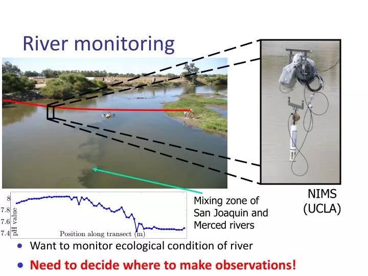
NIMS (UCLA). 8. 7.8. 7.6. pH value. 7.4. Position along transect (m). River monitoring. Want to monitor ecological condition of river Need to decide where to make observations!. Mixing zone of San Joaquin and Merced rivers. Observation Selection for Spatial prediction.

E N D
NIMS (UCLA) 8 7.8 7.6 pH value 7.4 Position along transect (m) River monitoring • Want to monitor ecological condition of river • Need to decide where to make observations! Mixing zone of San Joaquin and Merced rivers
Observation Selection for Spatial prediction • Gaussian processes • Distribution over functions (e.g., how pH varies in space) • Allows estimating uncertainty in prediction observations Prediction pH value Confidencebands Unobserved process Horizontal position
Entropy of uninstrumented locations after sensing Mutual Information[Caselton Zidek 1984] • Finite set of possible locations V • For any subset A µ V, can compute Want: A* = argmax MI(A) subject to |A| ≤ k • Finding A* is NP hard optimization problem Entropy of uninstrumented locations before sensing
Constant factor, ~63% Optimal solution The greedy algorithm for finding optimal a priori sets • Want to find: A* = argmax|A|=k MI(A) • Greedy algorithm: • Start with A = ; • For i = 1 to k • s* := argmaxs MI(A [ {s}) • A := A [ {s*} 4 2 1 5 3 Theorem [ICML 2005, with Carlos Guestrin, Ajit Singh] Result of greedy algorithm
¸ 20°C <20°C ¸ 18°C >15°C <18°C X12=? X23 =? MI(…) = 2.1 MI(…) = 2.4 Sequential design • Observed variables depend on previous measurements and observation policy • MI() = expected MI score over outcome of observations X5=17 X5=? X5=21 Observationpolicy X3 =16 X3 =? X2 =? X7 =19 X7 =? MI() = 3.1 MI(X5=17, X3=16, X7=19) = 3.4
A priori vs. sequential • Sets are very simple policies. Hence: maxA MI(A)·max MI() subject to |A|=||=k • Key question addressed in this work: How much better is sequential vs. a priori design? • Main motivation: • Performance guarantees about sequential design? • A priori design is logistically much simpler!
1 8 7.8 Correlation pH value 7.6 0.5 7.4 Position along transect (m) 0 4 2 0 2 4 Distance GPs slightly more formally • Set of locations V • Joint distribution P(XV) • For any A µ V, P(XA) Gaussian • GP defined by • Prior mean (s) [often constant, e.g., 0] • Kernel K(s,t) XV … … V Example: Squaredexponential kernel 1: Variance (Amplitude) 2: Bandwidth
Known parameters Known parameters (bandwidth, variance, etc.) Mutual Information does not depend on observed values: No benefit in sequential design! maxA MI(A) = max MI()
Unknown parameters Unknown (discretized) parameters: Prior P( = ) Mutual Information does depend on observed values! depends on observations! Sequential design can be better! maxA MI(A)·max MI()
Key result: How big is the gap? Gap depends on H() • If = known: MI(A*) = MI(*) • If “almost” known: MI(A*) ¼ MI(*) MI 0 MI(A*) MI(*) Theorem: MI of best policy MI of best param. spec. set As H() ! 0: MI of best policy Gap size MI of best set
Result of greedy algorithm Optimal seq. plan Gap ≈ 0 (known par.) ~63% Near-optimal policy if parameter approximately known • Use greedy algorithm to optimizeMI(Agreedy | ) = P() MI(Agreedy | ) • Note: • | MI(A | ) – MI(A) | · H() • Can compute MI(A | ) analytically, but not MI(A) Corollary [using our result from ICML 05]
Parameter entropybefore observing s P.E. after observing s Parameter info-gain exploration (IGE) • Gap depends on H() • Intuitive heuristic: greedily select s* = argmaxs I(; Xs) = argmaxs H() – H( | Xs) • Does not directly try to improve spatial prediction • No sample complexity bounds
Implicit exploration (IE) • Intuition: Any observation will help us reduce H() • Sequential greedy algorithm: Given previous observations XA = xA, greedily select s* = argmaxs MI ({Xs} | XA=xA, ) • Contrary to a priori greedy, this algorithm takes observations into account (updates parameters) Proposition: H( | X) · H() “Information never hurts” for policies No samplecomplexity bounds
Learning the bandwidth Can narrow down kernel bandwidth by sensing inside and outside bandwidth distance! Sensors outsidebandwidth are≈ independent Kernel Bandwidth A B C Sensors withinbandwidth arecorrelated
1 2 2 0 0 0.5 -2 -2 0 -4 -2 0 2 4 -2 0 2 -2 0 2 At this distance correlation gap largest Hypothesis testing:Distinguishing two bandwidths • Square exponential kernel: • Choose pairs of samples at distance to test correlation! BW = 3 BW = 1 Correlation under BW=1 Correlation under BW=3
Hypothesis testing:Sample complexity Theorem: To distinguish bandwidths with minimum gap in correlation and error < we need independent samples. • In GPs, samples are dependent, but “almost” independent samples suffice! (details in paper) • Other tests can be used for variance/noise etc. • What if we want to distinguish more than two bandwidths?
0.6 ) 0.4 q P( 0.2 0 1 2 3 4 5 Hypothesis testing:Binary searching for bandwidth • Find “most informative split” at posterior median Testing policy ITE needs only logarithmically many tests! Theorem: If we have tests with error < T then
Exploration—Exploitation Algorithm • Exploration phase • Sample according to exploration policy • Compute bound on gap between best set and best policy • If bound < specified threshold, go to exploitation phase, otherwise continue exploring. • Exploitation phase • Use a priori greedy algorithm select remaining samples • For hypothesis testing, guaranteed to proceed to exploitation after logarithmically many samples!
0.5 2 IE 0.45 More param. uncertainty 1.5 IGE 0.4 ITE 1 0.35 IE IGE 0.3 ITE 0.5 More observations 0 5 10 15 20 25 0 5 10 15 20 Results Temperature data • None of the strategies dominates each other • Usefulness depends on application IGE: Parameter info-gain ITE: Hypothesis testing IE: Implicit exploration More RMS error More observations
1 0 10 20 30 40 50 Coordinates (m) Nonstationarity by spatial partitioning • Isotropic GP for each region, weighted by region membership • spatially varying linear combination Nonstationary fit Stationary fit • Problem: Parameter space grows exponentially in #regions! • Solution: Variational approximation (BK-style) allows efficient approximate inference (Details in paper)
0.2 0.15 IE, isotropic 0.1 a priori, (13.10/0.03) (14.49/0.02) nonstationary 1 (14.54/0.04) (13.82/0.10) 0.05 IE, nonstationary 0 0 10 20 30 40 50 0 10 20 30 40 Coordinates (m) Results on river data • Nonstationary model + active learning lead to lower RMS error More RMS error Larger bars = later sample More observations
10 1.5 Random, nonstationary 9.5 IGE, IE nonstationary 9 nonstationary 8.5 1 IE, 8 isotropic 7.5 IE, IGE nonstationary 7 nonstationary 0.5 6.5 0 5 10 15 20 0 5 10 15 20 25 30 Results on temperature data • IE reduces error most quickly • IGE reduces parameter entropy most quickly More param. uncertainty More RMS error More observations More observations
Conclusions • Nonmyopicapproach towards active learning in GPs • If parameters known, greedy algorithm achieves near-optimal exploitation • If parameters unknown, perform exploration • Implicit exploration • Explicit, using information gain • Explicit, using hypothesis tests, with logarithmic sample complexity bounds! • Each exploration strategy has its own advantages • Can use bound to compute stopping criterion • Presented extensive evaluation on real world data