Download
1 / 17
170 likes | 288 Views
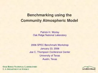
Scaling of the Community Atmospheric Model to ultrahigh resolution. Michael F. Wehner Lawrence Berkeley National Laboratory mfwehner@lbl.gov with Pat Worley (ORNL), Art Mirin (LLNL) Lenny Oliker (LBNL), John Shalf (LBNL). Motivations. First meeting of the WCRP Modeling Panel (WMP)

E N D
Scaling of the Community Atmospheric Model to ultrahigh resolution Michael F. Wehner Lawrence Berkeley National Laboratory mfwehner@lbl.gov with Pat Worley (ORNL), Art Mirin (LLNL) Lenny Oliker (LBNL), John Shalf (LBNL)
Motivations • First meeting of the WCRP Modeling Panel (WMP) • Convened at the UK MetOffice October, 2005 by Shukla • Discussion focused on benefits and costs of climate and weather models approaching 1km in horizontal resolution • Eventual white paper by Shukla and Shapiro for the WMO JSC • “Counting the Clouds”, A presentation by Dave Randall (CSU) to DOE SciDAC (June 2005) • Dave presents a compelling argument for global atmospheric models that resolve cloud systems rather than parameterize them. • Presentation is on the web at www.scidac.org
fvCAM • NCAR Community Atmospheric Model version 3.1 • Finite Volume hydrostatic dynamics (Lin-Rood) • Parameterized physics is the same as the spectral version • Our previous studies focus on the performance of the fvCAM with a 0.5oX0.625oX28L mesh on a wide variety of platforms (See Pat Worley’s talk this afternoon) • In the present discussion, we consider the scaling behavior of this model over a range of existing mesh configurations and extrapolate to ultra-high horizontal resolution.
Operations count • Exploit three existing horizontal resolutions to establish the scaling behavior of the number of operations per fixed simulation period. • Existing resolutions (all 28 vertical levels) • “B” 2oX2.5o • “C” 1oX1.25o • “D” 0.5ox0.625o • Define: • m = # of longitudes, n = # of latitudes
Operations Count (Scaling) • Parameterized physics • Time step can remain constant • Ops = m * n • Dynamics • Time step determined by the Courant condition • Ops = m * n * n • Filtering • Allows violation of an overly restrictive Courant condition near the poles • Ops = m * log(m) * n * n
Sustained computation rate requirements • A reasonable metric in climate modeling is that the model • must run 1000 times faster than real time. • Millenium scale control runs complete in a year. • Century scale transient runs complete in a month.
Can this code scale to these speeds? • Domain decomposition strategies • Np = number of subdomains, Ng = number of grid points • Existing strategy is 1D in the horizontal • A better strategy is 2D in the horizontal • Note: fvCAM also uses a vertical decomposition as well as OpenMP parallelism to increase utilization of processors.
Processor scaling • The performance data from fvCAM fits the first model well but tells us little about future technologies. • A practical constraint is that the number of subdomains is limited to be less than or equal to the number of horizontal cells . • At three cells across per subdomain, complete communication of the model’s data is required. • This constraint can provide an estimate of the maximum number of subdomains (~ processors) as well as the minimum processor performance required to achieve the 1000X real time metric (in the absence of communication costs).
Maximum number of horizontal subdomains -2,123,366 -3840
Minimum processor speed to achieve 1000X real time Assume no vertical decomposition and no OpenMP
Memory scales slower than processor speed due to Courant condition.
Strawman 1km climate computer • “I” mesh at 1000X real time • .015oX.02oX100L • ~10 Petaflops sustained • ~100 Terabytes total memory • ~2 million horizontal subdomains • ~10 vertical domains • ~20 million processors at 500Mflops each sustained • including communications costs. • 5 MB memory per processor • ~20,000 nearest neighbor send-receive pairs per subdomain per simulated hour of ~10KB each
Conclusions • fvCAM could probably be scaled up to a 1.5km mesh • Dynamics would have to be changed to fully non-hydrostatic • The scaling of the operations count is superlinear with horizontal resolution because of the Courant condition. • Surprisingly, filtering does not dominate the calculation. Physics cost is negligible. • One dimensional horizontal domain decomposition strategy will likely not work. • Limits on processor number and performance are too severe. • Two dimensional horizontal domain decomposition strategy would be favorable but requires a code rewrite. • Its not as crazy as it sounds.