Download
1 / 105
1.05k likes | 1.06k Views
Image Filtering and Edge Detection. ECE 847: Digital Image Processing. Stan Birchfield Clemson University. Motivation. Two closely related problems:. blur (to remove noise). differentiate (to highlight details).

E N D
Image Filteringand Edge Detection ECE 847:Digital Image Processing Stan Birchfield Clemson University
Motivation Two closely related problems: blur (to remove noise) differentiate (to highlight details) S. Birchfield, Clemson Univ., ECE 847, http://www.ces.clemson.edu/~stb/ece847
Motivation Two closely related problems: blur (to remove noise) differentiate (to highlight details) Underlying math is the same! S. Birchfield, Clemson Univ., ECE 847, http://www.ces.clemson.edu/~stb/ece847
Recall: Types of image transformations • Graylevel transformsI’(x,y) f( I(x,y) )(arithmetic, logical, thresholding, histogram equalization, …) • Geometric transformsI’(x,y) f( I(x’,y’) )(flip, flop, rotate, scale, …) • Area-based transformsI’(x,y) f( I(x,y), I(x+1,y+1), … )(morphological operators, convolution) • Global transformsI’(x,y) f( I(x’,y’), x’,y’ )(Fourier transform, wavelet transform) } filtering A S. Birchfield, Clemson Univ., ECE 847, http://www.ces.clemson.edu/~stb/ece847
Outline • Convolution • Gaussian convolution kernels • Smoothing an image • Differentiating an image • Canny edge detection • Laplacian of Gaussian
Linear time-invariant (LTI) systems • Systemproduces output from input: • Two properties of linear systems: • homogeneity (or scaling):Scaling of input propagates to output • superposition (or additivity):Sum of two inputs yields sum of two outputs • Time-invariant (or shift-invariant):Output does not depend upon absolute time (shift) of input S. Birchfield, Clemson Univ., ECE 847, http://www.ces.clemson.edu/~stb/ece847
System examples • Linear time invariant: y(t) = 5x(t) y(t) = x(t-1) + 2x(t) + x(t+1) • Linear time varying:y(t) = tx(t) • Nonlinear:y(t) = cos( x(t) ) S. Birchfield, Clemson Univ., ECE 847, http://www.ces.clemson.edu/~stb/ece847
Question • Is this system linear? y(t) = mx(t) + b S. Birchfield, Clemson Univ., ECE 847, http://www.ces.clemson.edu/~stb/ece847
Question • Is this system linear? y(t) = mx(t) + b • No, not if b ≠ 0, because scaling the input does not scale the output:m∙ax(t) + b = amx(t) + b ≠ ay(t) • Technically, this is called an affine system • Ironic that a linear equation does not describe a linear system S. Birchfield, Clemson Univ., ECE 847, http://www.ces.clemson.edu/~stb/ece847
LTI systems are described by convolution • Continuous • Discrete (Notation is usually *, but we want to avoid confusion with multiplication) Note: Convolution is commutative S. Birchfield, Clemson Univ., ECE 847, http://www.ces.clemson.edu/~stb/ece847
Relationship to cross-correlation • Continuous • Discrete complex conjugate no flip Note: Convolution and cross-correlation are identical when the signal is real and the kernel is symmetric S. Birchfield, Clemson Univ., ECE 847, http://www.ces.clemson.edu/~stb/ece847
Convolution with discrete,finite duration signals • width and half-width of kernel: • convolution assumes • examples: (if w is odd) (if w is odd) (underline indicates origin) S. Birchfield, Clemson Univ., ECE 847, http://www.ces.clemson.edu/~stb/ece847
Convolution implementation (1D) • In memory, indices must be non-negative • So shift kernel by : • Algorithm: • Flip g (not needed in practice) • For each x • Align g so that center is at x • Sum the products S. Birchfield, Clemson Univ., ECE 847, http://www.ces.clemson.edu/~stb/ece847
Kernel flipping • In practice, no need to flip g • If g is symmetric, then same result [ 1 2 1 ] • If g is antisymmetric, then just sign change [ -1 0 1 ] • For real images and symmetric kernels, convolution = cross-correlation S. Birchfield, Clemson Univ., ECE 847, http://www.ces.clemson.edu/~stb/ece847
Convolution implementation (1D) • Algorithm: • Note: • Convolution cannot be done “in place” • Output must be separate from input, to avoid corrupting computation S. Birchfield, Clemson Univ., ECE 847, http://www.ces.clemson.edu/~stb/ece847
1D convolution example • Given the 1D signal • Suppose we want to compute the average of each pixel and its 2 neighbors • Solution: slide kernel across signal, elementwise multiplication and sum : • Result: • This is known as shift-multiply-add S. Birchfield, Clemson Univ., ECE 847, http://www.ces.clemson.edu/~stb/ece847
Signal borders • Zero extension: [1 5 6 7] * [1/3 1/3 1/3] is the same as [… 0 1 5 6 7 0 …] * [… 0 1 1 1 0 …]/3 • Result: [… 0 0 0 0.33 2 4 6 4.33 2.33 0 0 0 …] • If signal has length n and kernel has length w, then result has length n+w-1 • But we adopt convention of cropping output to same size as input S. Birchfield, Clemson Univ., ECE 847, http://www.ces.clemson.edu/~stb/ece847
1D convolution example (replication/ reflection) kernel image 16 8 * ¼(8) + ½(8) + ¼(24) = 12 (flipped) ¼(8) + ½(24) + ¼(48) = 26 = 12 26 38 32 20 ¼(48) + ½(32) + ¼(16) = 32 ¼(32) + ½(16) + ¼(16) = 20 S. Birchfield, Clemson Univ., ECE 847, http://www.ces.clemson.edu/~stb/ece847
Algorithm: kernel is a little image containing weights Algorithm: Flip g (horizontally and vertically – not important in practice) For each (x,y) Align g so that center is at (x,y) Sum the products Convolution in 2D image convolution kernel (shifted by and ) S. Birchfield, Clemson Univ., ECE 847, http://www.ces.clemson.edu/~stb/ece847
Convolution implementation (2D) • Algorithm: • Again, note that convolution cannot be done “in place” S. Birchfield, Clemson Univ., ECE 847, http://www.ces.clemson.edu/~stb/ece847
Convolution as matrix multiplication • Equivalent to multiplying by Toeplitz matrix (ignoring border effects): • Applicable to any dimension extend by replication S. Birchfield, Clemson Univ., ECE 847, http://www.ces.clemson.edu/~stb/ece847
Convolution as Fourier multiplication • Convolution in spatial domain is multiplication in frequency domain • Computationally efficient only when kernel is large • Equivalent to circular convolution (signals are treated as periodic) S. Birchfield, Clemson Univ., ECE 847, http://www.ces.clemson.edu/~stb/ece847
Outline • Convolution • Gaussian convolution kernels • Smoothing an image • Differentiating an image • Canny edge detection • Laplacian of Gaussian
Two types of convolution kernels Smoothing (Smoothing a constant function should not change it)Example: (1/3) * [1 1 1]Lowpass filter (Gaussian) Differentiating (Differentiating a constant function should return 0) Example: (1/2) * [-1 0 1] Highpass filter(derivative of Gaussian) … also bandpass filters (Laplacian of Gaussian) S. Birchfield, Clemson Univ., ECE 847, http://www.ces.clemson.edu/~stb/ece847
Box filter Simplest smoothing kernel is the box filter: 1/n 0 (n=1) (n=3) (n=5) Odd length avoids undesirable shifting of signal S. Birchfield, Clemson Univ., ECE 847, http://www.ces.clemson.edu/~stb/ece847
Gaussian kernel • Gaussian function is “bell curve”: • Performs weighted average of neighboring values mean (center) standard deviation (width) variance Normalization factor ensures PDF:
Gaussian Why is Gaussian so important? • completely described by 1st and 2nd order statistics • central limit theorem • localized in space and frequency • convolution of two Gaussians is Gaussianm=m1+m2 and s2=s12+s22 • separable (efficient) Gaussian provides weighted average of neighbors S. Birchfield, Clemson Univ., ECE 847, http://www.ces.clemson.edu/~stb/ece847
Repeated averaging Repeated convolution with box filter yields convolution with Gaussian (from Central Limit Theorem): These are the odd rows of the binomial (Pascal’s) triangle: (2k+1)th row approximates Gaussian with s2=k/2 Note that scale factor is power of two (makes normalization fast because division is just bit shift) k=1, s2=0.5, s=0.7 k=2, s2=1, s=1 S. Birchfield, Clemson Univ., ECE 847, http://www.ces.clemson.edu/~stb/ece847
Repeated averaging (cont.) Trinomial triangle also yields Gaussian approximations: kth row approximates Gaussian with s2=2k/3 Example: In general, n repeated convolutions with s2Gaussian approximates single convolution with ns2 Gaussian S. Birchfield, Clemson Univ., ECE 847, http://www.ces.clemson.edu/~stb/ece847
Computing the variance of a smoothing kernel • Set of values: • Mean is • Variance is deviation from mean:
Computing the variance of a smoothing kernel • Kernel is a sequence of values: • Is this the mean? • Is this the variance? No, because a sequenceis not a set (order matters)
Computing the variance of a smoothing kernel • Kernel is a sequence of values: • Mean: • Variance: Note: These are weighted averages, with weightsg(i)
Example • Kernel: • Mean: • Variance: g[0] g[1] g[2] 2 1 1 Note: 0 1 2
Building a Gaussian kernel • How to build Gaussian kernel with arbitrary s? • Sample continuous Gaussian continuous normalization f=2.5 is reasonable, to capture ±2.5s, because discrete version approximately captures But we want to ensure discrete normalization S. Birchfield, Clemson Univ., ECE 847, http://www.ces.clemson.edu/~stb/ece847
Common Gaussian kernels (The subscript is s2.)
Sampling effects • Resulting discrete function will not have the same s as original continuous function • Example: • Sample s=1 (s2=1) (0.4026) * [0.1353 0.6065 1.0000 0.6065 0.1353] • Resulting discrete kernel has s2=(0.4026) * 2 * [(0.1353)*(22)+(0.6065)*(12)] = 0.92 • Another example: • Sample s=1.08 (s2=1.17) (0.3755) * [0.1800 0.6514 1.0000 0.6514 0.1800]\approx (1/16) [ 1 4 6 4 1 ] • Resulting discrete kernel has s=1 S. Birchfield, Clemson Univ., ECE 847, http://www.ces.clemson.edu/~stb/ece847
(Some say) three samples is not enough to capture Gaussian Spatial domain: Capture 98.76% of the area with ±2.5s (continuous) kernel width = 2*(halfwidth)+1 Frequency domain: Capture 98.76% of the area with But in practice three samples is common (Note: sampling at 1 pixel intervals cutoff frequency is 2p(0.5) = ±p) [Trucco and Verri, p. 60] S. Birchfield, Clemson Univ., ECE 847, http://www.ces.clemson.edu/~stb/ece847
What is the best 3x1 Gaussian kernel? Spatial domain: Capture some percentage of the area with ±as w ≥ 2as kernel width = 2*(halfwidth)+1 Frequency domain: Capture the same percentage withCombining these yields: 2a/s ≤ 2p • = 0.69 a = 2.17 97% of Gaussian is captured (not bad!) S. Birchfield, Clemson Univ., ECE 847, http://www.ces.clemson.edu/~stb/ece847
Binomial triangle Gaussians are too wide Recall that the binomial (Pascal’s) triangle is an easy way to construct a Gaussian of width (2k+1) and variance s2=k/2 Recall that to capture 98.76% of the area, we want For s = 1.0, width is perfect, but for larger s the kernel is too wide What are the implications for repeated averaging? S. Birchfield, Clemson Univ., ECE 847, http://www.ces.clemson.edu/~stb/ece847
Outline • Convolution • Gaussian convolution kernels • Smoothing an image • Differentiating an image • Canny edge detection • Laplacian of Gaussian
Separability Can alwaysconstruct 2D kernel by convolving 1D kernels: Some 2D kernels can be decomposed into 1D kernels: A 2D kernel is separable iff all rows / columns are linearly dependent S. Birchfield, Clemson Univ., ECE 847, http://www.ces.clemson.edu/~stb/ece847
Separability Separable convolution is less expensive: O(n^2) operations O(2n) operations Allowed because convolution is associative: Convolve with two 1D kernels instead of one 2D kernel S. Birchfield, Clemson Univ., ECE 847, http://www.ces.clemson.edu/~stb/ece847
Separability of Gaussian 2D Gaussian (isotropic): Convolution with 2D Gaussian is same as convolution with two 1D Gaussians (horizontal and vertical): S. Birchfield, Clemson Univ., ECE 847, http://www.ces.clemson.edu/~stb/ece847
Separable convolution horizontal then vertical (or vice versa) input output temporary Remember: Do not try to perform convolution in place! S. Birchfield, Clemson Univ., ECE 847, http://www.ces.clemson.edu/~stb/ece847
Smoothing with a Gaussian from http://www-static.cc.gatech.edu/classes/AY2007/cs4495_fall/html/materials.html
Effects of different sigmas from http://www-static.cc.gatech.edu/classes/AY2007/cs4495_fall/html/materials.html
Gaussian pyramid smooth downsample s Shannon’s sampling theorem: After smoothing, many pixels are redundant. Therefore, we can discard them (by downsampling) without losing information from http://www-static.cc.gatech.edu/classes/AY2007/cs4495_fall/html/materials.html