Download
1 / 75
780 likes | 1.02k Views
Image Filtering. Overview of Filtering. Convolution Gaussian filtering Median filtering. Overview of Filtering. Convolution Gaussian filtering Median filtering. Motivation: Noise reduction. Given a camera and a still scene, how can you reduce noise?.

E N D
Overview of Filtering • Convolution • Gaussian filtering • Median filtering
Overview of Filtering • Convolution • Gaussian filtering • Median filtering
Motivation: Noise reduction • Given a camera and a still scene, how can you reduce noise? Take lots of images and average them! What’s the next best thing? Source: S. Seitz
Moving average 1 1 1 1 1 1 1 1 1 “box filter” • Let’s replace each pixel with a weighted average of its neighborhood • The weights are called the filter kernel • What are the weights for the average of a 3x3 neighborhood? Source: D. Lowe
Defining Convolution f • Let f be the image and g be the kernel. The output of convolving f with g is denoted f * g. • Convention: kernel is “flipped” • MATLAB: conv2 (also imfilter) Source: F. Durand
Key properties • Linearity: filter(f1 + f2 ) = filter(f1) + filter(f2) • Shift invariance: same behavior regardless of pixel location: filter(shift(f)) = shift(filter(f)) • Theoretical result: any linear shift-invariant operator can be represented as a convolution
Properties in more detail • Commutative: a * b = b * a • Conceptually no difference between filter and signal • Associative: a * (b * c) = (a * b) * c • Often apply several filters one after another: (((a * b1) * b2) * b3) • This is equivalent to applying one filter: a * (b1 * b2 * b3) • Distributes over addition: a * (b + c) = (a * b) + (a * c) • Scalars factor out: ka * b = a * kb = k (a * b) • Identity: unit impulse e = […, 0, 0, 1, 0, 0, …], a * e = a
Annoying details • What is the size of the output? • MATLAB: conv2(f, g,shape) • shape = ‘full’: output size is sum of sizes of f and g • shape = ‘same’: output size is same as f • shape = ‘valid’: output size is difference of sizes of f and g full same valid g g g g f f f g g g g g g g g
Annoying details • What about near the edge? • the filter window falls off the edge of the image • need to extrapolate • methods: • clip filter (black) • wrap around • copy edge • reflect across edge Source: S. Marschner
Annoying details • What about near the edge? • the filter window falls off the edge of the image • need to extrapolate • methods (MATLAB): • clip filter (black): imfilter(f, g, 0) • wrap around: imfilter(f, g, ‘circular’) • copy edge: imfilter(f, g, ‘replicate’) • reflect across edge: imfilter(f, g, ‘symmetric’) Source: S. Marschner
Practice with linear filters 0 0 0 0 1 0 0 0 0 ? Original Source: D. Lowe
Practice with linear filters 0 0 0 0 1 0 0 0 0 Original Filtered (no change) Source: D. Lowe
Practice with linear filters 0 0 0 0 0 1 0 0 0 ? Original Source: D. Lowe
Practice with linear filters 0 0 0 0 0 1 0 0 0 Original Shifted left By 1 pixel Source: D. Lowe
Practice with linear filters 1 1 1 1 1 1 1 1 1 ? Original Source: D. Lowe
Practice with linear filters 1 1 1 1 1 1 1 1 1 Original Blur (with a box filter) Source: D. Lowe
Practice with linear filters 0 1 0 1 0 1 1 0 2 1 0 1 1 0 1 0 0 1 - ? (Note that filter sums to 1) Original Source: D. Lowe
Practice with linear filters 0 1 0 1 0 1 1 0 2 1 0 1 1 0 1 0 0 1 - Original • Sharpening filter • Accentuates differences with local average Source: D. Lowe
Sharpening before after Slide credit: Bill Freeman
Spatial resolution and color R G B original Slide credit: Bill Freeman
R G B Blurring the G component processed original Slide credit: Bill Freeman
R G B Blurring the R component processed original Slide credit: Bill Freeman
R G B processed Blurring the B component original Slide credit: Bill Freeman
From W. E. Glenn, in Digital Images and Human Vision, MIT Press, edited by Watson, 1993 Slide credit: Bill Freeman
Lab color components L A rotation of the color coordinates into directions that are more perceptually meaningful: L: luminance, a: red-green, b: blue-yellow a b Slide credit: Bill Freeman
L a b processed Blurring the L Lab component original Slide credit: Bill Freeman
L a b processed Blurring the a Lab component original Slide credit: Bill Freeman
L a b processed Blurring the b Lab component original Slide credit: Bill Freeman
Overview of Filtering • Convolution • Gaussian filtering • Median filtering
Smoothing with box filter revisited • Smoothing with an average actually doesn’t compare at all well with a defocused lens • Most obvious difference is that a single point of light viewed in a defocused lens looks like a fuzzy blob; but the averaging process would give a little square Source: D. Forsyth
Smoothing with box filter revisited • Smoothing with an average actually doesn’t compare at all well with a defocused lens • Most obvious difference is that a single point of light viewed in a defocused lens looks like a fuzzy blob; but the averaging process would give a little square • Better idea: to eliminate edge effects, weight contribution of neighborhood pixels according to their closeness to the center, like so: “fuzzy blob” Source: D. Forsyth
Gaussian Kernel • Constant factor at front makes volume sum to 1 (can be ignored, as we should re-normalize weights to sum to 1 in any case) 0.003 0.013 0.022 0.013 0.003 0.013 0.059 0.097 0.059 0.013 0.022 0.097 0.159 0.097 0.022 0.013 0.059 0.097 0.059 0.013 0.003 0.013 0.022 0.013 0.003 5 x 5, = 1 Source: C. Rasmussen
Choosing kernel width • Gaussian filters have infinite support, but discrete filters use finite kernels Source: K. Grauman
Choosing kernel width • Rule of thumb: set filter half-width to about 3 σ
Gaussian filters • Remove “high-frequency” components from the image (low-pass filter) • Convolution with self is another Gaussian • So can smooth with small-width kernel, repeat, and get same result as larger-width kernel would have • Convolving two times with Gaussian kernel of width σ is same as convolving once with kernel of width σ√2 • Separable kernel • Factors into product of two 1D Gaussians Source: K. Grauman
Separability of the Gaussian filter Source: D. Lowe
* = = * Separability example 2D convolution(center location only) The filter factorsinto a product of 1Dfilters: Perform convolutionalong rows: Followed by convolutionalong the remaining column: For MN image, PQ filter: 2D takes MNPQ add/times, while 1D takes MN(P + Q) Source: K. Grauman
Overview of Filtering • Convolution • Gaussian filtering • Median filtering
Alternative idea: Median filtering • A median filter operates over a window by selecting the median intensity in the window • Is median filtering linear? Source: K. Grauman
Median filter Replace each pixel by the median over N pixels (5 pixels, for these examples). Generalizes to “rank order” filters. Median([1 7 1 5 1]) = 1 Mean([1 7 1 5 1]) = 2.8 Spike noise is removed In: Out: 5-pixel neighborhood Monotonic edges remain unchanged In: Out:
Median filtering results Best for salt and pepper noise http://homepages.inf.ed.ac.uk/rbf/HIPR2/mean.htm#guidelines
Median vs. Gaussian filtering 3x3 5x5 7x7 Gaussian Median
Edges http://todayinart.com/files/2009/12/500x388xblind-contour-line-drawing.png.pagespeed.ic.DOli66Ckz1.png
Edge detection • Goal: Identify sudden changes (discontinuities) in an image • Intuitively, most semantic and shape information from the image can be encoded in the edges • More compact than pixels • Ideal: artist’s line drawing (but artist is also using object-level knowledge) Source: D. Lowe
Origin of edges • Edges are caused by a variety of factors: surface normal discontinuity depth discontinuity surface color discontinuity illumination discontinuity Source: Steve Seitz
Edges in the Visual Cortex • Extract compact, generic, representation of image that carries sufficient information for higher-level processing tasks • Essentially what area V1 does in our visual cortex. http://www.usc.edu/programs/vpl/private/photos/research/retinal_circuits/figure_2.jpg
Image gradient • The gradient of an image: The gradient points in the direction of most rapid increase in intensity • How does this direction relate to the direction of the edge? The gradient direction is given by The edge strength is given by the gradient magnitude Source: Steve Seitz