Download
1 / 31
320 likes | 440 Views
Observation representativeness error ECMWF model spectra Application to ADM sampling mode and Joint-OSSE. Motivation. ESA is re-considering burst vs. continuous mode for ADM-Aeolus Information content of various sampling modes for NWP Effective model resolution

E N D
Observation representativeness errorECMWF model spectraApplication to ADM sampling modeand Joint-OSSE
Motivation • ESA is re-considering burst vs. continuous mode for ADM-Aeolus • Information content of various sampling modes for NWP • Effective model resolution • Number of degrees of freedom of a model • ADM observation representation • Observations should represent this model resolution • ADM representativeness error
observation Data assimilation Atmospheric analysis NWP model Observation weight in data assimilation • Observation impact in atmospheric analysis is determined by the relative weight of the observation and the model in the analysis
Perfect observation • Perfect observation has no observation error: R=0 • For simplicity, assume the observation directly related to a model parameter and located on a model grid point: H=I • K=I • y = Hxt + = xt (no observation error is assumed) • xa=xb+I(xt-xb) = xt • The analysed state equals the true atmospheric state at the measurement location • Sounds good ……….. or?
Perfect observation The model state is a smooth representation of the real atmospheric state • Model perfectly fits observation, but no constraint elsewhere (overfitting) assimilation of perfect observation
Perfect observation • What goes wrong? • Model information (including information from observations in previous cycles) is ignored • Model is forced to fit the small-scale structures present in the (point) observation • But • model is a smooth representation of the real atmosphere, not representing small-scale features • Small-scale structures are not well treated by the model (noise) and should be avoided in the NWP analysis step. • Weight given to the observation is too large • How to determine a more appropriate weight?
Observation representativeness error • Representativeness error = the small scale atmospheric variability which is sampled by individual observations, but which the model is incapable of representing • To avoid ingesting small-scale structures in the model state, the impact (weight) of the observation in the analysis is reduced by increasing the observation error with the representativeness error, i.e., • observation error variance = measurement error variance + representativeness error variance. • How to determine the observation representativeness error?
k-3 5000 km cyclones 500 km k-5/3 2 km shifted Wave number spectra near tropopause Nastrom and Gage (1985) GASP aircraft data near tropopause • Wind spectra follow a • k-5/3 spectrum for horizontal • spatial scales below 500 km • atmospheric variability (m2s-2) is found by the surface below the spectrum
1000 hPa 500 hPa ECMWF model spectra Lorenc curve (1992): k-5/3 atmosphere wind variability spectrum (ESA study by Lorenc on ADM) based on Nastrom and Gage Power law and amplitude determine unresolved model variance ECMWF (2008, T799) ECMWF model does not well resolve the atmospheric variability on scales smaller than ~300 km
Illustration representativeness error model • Resolved wind variability: ECMWF and scatterometer Jur Vogelzang (2006)
Tropical cyclone Ike HARMONIE ECMWF T799 ~ 25 km More small-scale structures in high-resolution (LAM) models HARMONIE ~ 2.5 km
Implication for Joint OSSE • Nature run (NR): ECMWF T511/T799 • Lacking atmospheric variability on scales smaller than ~250km • Simulate atmospheric variability for missing NR scales • representativeness error • Observation simulation: o = intpol(NR) + instrument error + representativeness error
Model resolution cell • Introduce Model Resolution Cell (MRC): • spatial scales below the MRC are not well resolved by the model • ECMWF model: MRC ~250km • unresolved wind variability: • UKMO 1992: unresolved wind variability: 3.95 m2s-2 computational grids of global NWP models have increased substantially over the last 15 years, but the horizontal scales that are resolved by these models have increased to a much lesser extent
ADM representativeness error burst mode • Assumption: along and across track variabilities are independent and of equal size • Total error error variance o 2 = r2across + r2along + m2/N MRC along track across track representativeness error continuous mode instrument error ~ photon counts with r2 = atmospheric variability in MRC MRC Increasing the sample length reduces the along track representativeness error !
ADM information content • Analysis equations Observation impact [0,1]; 0: no impact, 1: maximum impact (analysis equals true atmosphere)
Numerical example • Square model area of 2,500 km2, 25 km model grid, 10000 model grid points • single layer at 500 hPa • No clouds B b = 2.5 ms-1 LB = 250 km
Numerical example (2) – burst mode A R sampling Observation impact = 0.52
ADM continuous mode • Pulse repetition frequency: 50 Hz (100 Hz for burst mode) • Same energy per shot • Double the energy along a 200 km track in continuous mode • Continuous mode offers more flexibility • 50/100/200/ …. km accumulation • 50/100/200/ …. km observation distance • Increasing the accumulation length reduces the representativeness error • BUT, observation correlation increases with decreasing observation distance
A R sampling Numerical example (3) – continuous mode 100 km accumulation, 100 km spacing observation impact = 0.61 200 km accumulation, 200 km spacing observation impact = 0.63 50 km accumulation, 50 km spacing observation impact = 0.60 Closely separated observations => highly correlated => reduced impact
LAM model resolving small-scales • Assume that models ARE capable to resolve 50 km scales; LB=50 km
LAM model resolving small-scales – ctd. 0.24 0.50 Models capable of resolving small-scale structures => high effective model resolution => small representativeness errors, closely separated observations are less correlated => continuous mode substantially better than burst mode
Conclusion • Spatial scales that can be resolved by global NWP models has not decreased a lot over the last 15 years; model resolution cell ~ 250 – 300 km • Burst mode is still a useful scenario, despite the increased model grid resolution • 100 km accumulations provide independent information on model degrees of freedom (model resolution cells) • The quality of ADM-Aeolus HLOS winds is expected to be better, on average, in continuous mode than in burst mode • About double the energy is transmitted into the atmosphere • Similar instrument noise (for 100 km accumulation) • Reduced representativeness error • Continuous mode offers a variety of accumulation scenarios (possibly depending on cloud coverage) • More advanced processing needed to get the maximum out of it
Effective model resolution • Effective model resolution is not the same as model grid mesh size • Effective model resolution is related to the spatial scales that can be resolved by the model Model grid mesh size ECMWF 1992: 100 km grid box ECMWF 2008: 25 km grid box ECMWF 2010: 15 km grid box
Model resolution cell/representativeness error summary • Model resolution ~ number of degrees of freedom of the model • Number of degrees of freedom is limited because • Limited computer capacity • Limited observation coverage to measure atmosphere non-linearity • model is a smooth representation of the real atmosphere, not representing small-scale features area (MRC) mean variables (model of a model) • Small-scale structures are not well treated by the model (noise) and should be avoided in the NWP analysis step. • Observations should “feed” these degrees of freedom, i.e. the area mean model variables • Observed scales smaller than the MRC (model resolution cell) are treated as noise, i.e. the representativeness error Representativeness error small scale variability which is sampled by an observation, but which the model is incapable of representing
Lorenc curve Model resolution (3) • Wind component variability • integration of the spectra in the previous image Model resolution cell (MRC) spatial scales below the MRC are not well resolved by the model MRC computational grids of global NWP models have increased substantially over the last 15 years, but the horizontal scales that are resolved by these models have increased to a much lesser extent
ADM representativeness error (2) • Numerical example ADM HLOS error: • ADM burst mode: sample length = 50 km • ADM continuous mode : sample length = 100, 170 km • m2/14 = 1.64 (ms-1)2 ~ 1 ms-1 LOS observation error standard deviation • r2 = 3.3 (ms-1)2 • MRC = 250 km
ADM impact • doubling of the energy in continuous mode does not double the additional impact as compared to burst mode. • Observation correlation reduces impact of individual observations (redundancy of sampling the degrees of freedom) • Highly correlated observations (last row) should be avoided