3D Numerical Simulations of Thermohaline Mixing in Low-Mass Red Giants

1. 3D Numerical Simulations of Thermohaline Mixing in Low-Mass Red Giants PavelDenisenkov, UVic

2. 3D Numerical Simulations of Thermohaline Mixing in Low-Mass Red Giants A story about how important and difficult it is to take account of mixing in stars when studying stellar nucleosynthesis PavelDenisenkov, UVic

3. The abundance of 3He should have increased by an order of magnitude since the Big Bang Nucleosynthesis, but it has been remaining nearly constant (From Bania, T. M., Rood, R. T., and Balser, D. S. 2007, Space Science Review, 130, 53)

4. The incomplete pp-chain reactions produce a lot of 3He far from the centre of a low-mass star on the main sequence, and low-mass stars are the most abundant species of stellar populations

5. Left:Evolution of a low-mass star in the HR diagram (M = 0.83M , Z = 0.0015) Right: Changes of abundance profiles inside the star that drive its evolution Data points are field stars with M = 0.8 – 0.9M, Z = 0.0005 – 0.002 from Gratton et al. (2000) Arrow in the right panel shows the bottom of convective envelope

6. Left:Evolution of a low-mass star in the HR diagram (M = 0.83M , Z = 0.0015) Right: Changes of abundance profiles inside the star that drive its evolution • on the MS, 3He is produced in a wide pocket (blue curve in the right panel) • after the MS, convection spreads 3He all over the envelope (the 1st dredge-up) • mass-loss on the RGB and AGB will deliver this 3He into ISM

7. Left:Evolution of a low-mass star in the HR diagram (M = 0.83M , Z = 0.0015) Right: Changes of abundance profiles inside the star that drive its evolution • on the MS, 3He is produced in a wide pocket (blue curve in the right panel) • after the MS, convection spreads 3He all over the envelope (the 1st dredge-up) • mass-loss on the RGB and AGB will deliver this 3He into ISM

8. How to explain the fact that the abundance of 3He in the ISM has not changed since the BBN? Low-mass red-giant-branch (RGB) stars show evidence of extra-mixing operating in their radiative zones between the hydrogen-burning shell and convective envelope that starts above the so-called “bump luminosity”. This RGB extra-mixing is most likely to reduce the envelope 3He abundance back to its BBN value.

9. What happens at the bump luminosity? Left:Evolution in the HRD around the bump luminosity (M = 0.83M , Z = 0.0015) Right: H-burning shell erases abundance discontinuities

10. What happens at the bump luminosity? Left:Evolution in the HRD around the bump luminosity (M = 0.83M , Z = 0.0015) Right: H-burning shell erases abundance discontinuities

11. What happens at the bump luminosity? Left:Evolution in the HRD around the bump luminosity (M = 0.83M , Z = 0.0015) Right: H-burning shell erases abundance discontinuities On upper RGB, above the bump luminosity, the radiative zone has uniform chemical composition, which facilitates fluid buoyancy of any origin

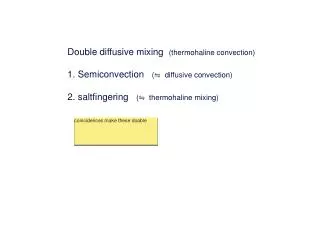
12. Thermohaline convection as a mechanism for extra mixing in RGB stars Thermohaline convection is driven by a small difference in salinity S between a fluid element and its surrounding medium when the atomic diffusivity  is much lower than the heat diffusivity K. In the ocean, it develops when both S and T decrease with depth and it takes a form of salt fingers, hence “salt-fingering convection” is another term for it. P( µ*, ρ1*,T) Reaction 3He(3He,2p)4He decreases µ locally byΔµ≈ −0.0001 Double-diffusive (K) instability leads to growing salt fingers in water

13. Thermohaline convection as a mechanism for extra mixing in RGB stars The RGB thermohaline convection is driven by a small difference in µ between a fluid parcel and its surrounding medium because the atomic diffusivity  is much lower than the heat diffusivity K. It develops when µ decreases with depth (usually, µ increases with depth in stars) Reaction 3He(3He,2p)4He decreases µ locally byΔµ≈ −0.0001

14. Thermohaline convection as a mechanism for extra mixing in RGB stars The RGB thermohaline convection is driven by a small difference in µ between a fluid parcel and its surrounding medium because the atomic diffusivity  is much lower than the heat diffusivity K. It develops when µ decreases with depth (usually, µ increases with depth in stars)

15. Thermohaline convection as a mechanism for extra mixing in RGB stars The RGB thermohaline convection is driven by a small difference in µ between a fluid parcel and its surrounding medium because the atomic diffusivity  is much lower than the heat diffusivity K. It develops when µ decreases with depth (usually, µ increases with depth in stars) Reaction 3He(3He,2p)4He decreases µ locally by |Δµ | ‹ 0.0001 (Eggleton et al. 2006)

16. 2D numerical simulations of thermohaline convection in the oceanic and RGB cases (a change of color from red to blue corresponds to an increase of S and µ) Salinity field Mean molecular weight field

17. 3D numerical simulations of the oceanic and RGB thermohaline convection Ocean (S) RGB (µ)

18. The empirically constrained rate of RGB extra-mixing is Dµ ≈ 0.01K which is a factor of 50 higher than the value estimated in our 2D and 3D numerical simulations • Therefore, the physical mechanism of RGB extra-mixing is most likely to be different from thermohaline convection driven by 3He burning • A promising alternative mechanism is the buoyant rise of magnetic flux rings (Parker’s instability)

19. The End