Download
1 / 22
220 likes | 378 Views
3D Numerical Simulations of Shear-Driven Atmospheric Turbulence. Joe Werne, Dave Fritts, Reg Hill Colorado Research Associates Division (CoRA) NorthWest Research Associates, Inc. (NWRA) Paul Bernhardt Naval Research Laboratory. Turbulence in Stably Stratified Environments.

E N D
3D Numerical Simulations of Shear-Driven Atmospheric Turbulence Joe Werne, Dave Fritts, Reg Hill Colorado Research Associates Division (CoRA) NorthWest Research Associates, Inc. (NWRA) Paul Bernhardt Naval Research Laboratory
Turbulence in Stably Stratified Environments Two processes dominate turbulence generation in stable stratification: • Wind-shear instability • Gravity-wave breaking The resulting turbulence is • Temporally episodic • Spatially intermittent (inhomogeneous and anisotropic) • Nearly all subgrid-scale At lower altitudes, measurements reveal and help quantify the dominant processes. These measurements include: • Cloud imagery • Balloon (rawinsonde) data • Aircraft data • Radar measurements
O(0.1-1km) Clear Air Turbulence: Wind Shear Estes Park, Colorado, 1979 (photo by Bob Perney)
Stably Stratified Dynamics Simulations Wind Shear Gravity-Wave Breaking U=Uotanh(z/h) T = αz
Stably Stratified Dynamics Simulations wind shear U=Uotanh(z/h) T = αz Ri = N2 h2/Uo2 Re=Uoh/ν Pe=Uoh/κ
Stably Stratified Dynamics Simulations wind shear wind shear asymptotic linear stability U=Uotanh(z/h) Note: ν = μ / ρ and ρ = ρ0 exp(z/H) ν increases by 105 from z=20km to 100km. Shear turbulence is easier to resolve in the mesosphere than in the stratosphere. Ri kx2 Ri = N2 h2/Uo2 Re=Uoh/ν Pe=Uoh/κ
PE 7 PE 6 FFT PE 5 PE 7 PE 6 PE 4 Z PE 5 PE 3 PE 4 Kx PE 2 PE 3 PE 2 PE 1 PE 1 PE 0 PE 0 Y Ky Kz X DNS-Code Details • Stream-function/vorticity formulation (T, W, ω3) • Fully spectral (3D FFT’s = 75% computation) • Radix 2,3,4,5 FFT’s • Spectral modes and NCPUs must be commensurate • Communication: MPI or shmem, global transpose • Parallel I/O every ~ 60 δt
Re=2500 (ReL=30,000) Ri=0.05 3000 x 1500 x 1500 spectral modes vorticity magnitude, side view
Re=2500 (ReL=30,000) Ri=0.05 3000 x 1500 x 1500 spectral modes vorticity magnitude, side view
Re=2500 (ReL=30,000) Ri=0.05 3000 x 1500 x 1500 spectral modes vorticity magnitude, top view of midplane
Re=2500 (ReL=30,000) Ri=0.05 3000 x 1500 x 1500 spectral modes vorticity magnitude, top view of midplane
Re=2500 (ReL=12,000) Ri=0.20 2000 x 1000 x 1000 spectral modes vorticity magnitude, side view
Re=2500 (ReL=12,000) Ri=0.20 2000 x 1000 x 1000 spectral modes vorticity magnitude, side view
Re=2500 (ReL=12,000) Ri=0.20 2000 x 1000 x 1000 spectral modes vorticity magnitude, top view of midplane
Re=2500 (ReL=12,000) Ri=0.20 2000 x 1000 x 1000 spectral modes vorticity magnitude, top view of midplane
Computed T, CT2, Ri profiles agree with rawinsonde observations. Low-Ri solutions consistent with cloud images. High-Ri solutions consistent with aircraft cliff-ramp measurements. Spectral slopes between -5/3 and -7/5, consistent with recent aircraft data 2nd-order structure function fits agree with aircraft and tower data consistent with atmospheric measurements DNS Rawinsonde Kolmogorov predicts 1.33 CT2 T Ri CT2 T Ri Validation of DNS Solutions Rescaled numerical solutions (with Re=104-105) are relevant to atmospheric shear layers (even when Re=107-108). Mesospheric simulations are much easier to resolve.
Uy (m/s) Relative Altitude (km) Ux (m/s) β = 0 β = 0.5 β = 1 Mesospheric Simulations Good News: • Reduced density means lower Re, which is easier to resolve New Twist: • Local wind profile can take the form of turning shear: u(z) = U0 tanh(z/h) v(z) = V0 sech(z/h)
Stratospheric Shear-Layer Census Data L ΔU ΔT z Re Ri
Turning-shear run matrix Re=300 Ri
vorticity magnitude 360×360×361 modes Re=300 Ri=0.05 β=0 Re=300 Ri=0.05 β=1 side view Ri top view
vorticity magnitude 360×360×361 modes Re=300 Ri=0.15 β=0 Re=300 Ri=0.15 β=1 side view Ri top view
Conclusions 1. Dramatically different turbulence dynamics and flow morphology result for weakly and strongly stratified wind shear. 2. Turning shear significantly affects instability dynamics and evolution. 3. Ramifications for transport and mixing? Ongoing & Future Work 1. Construct atmospheric Ri, Re, and β census PDFs using available observational data. 2. Generalize linear stability analysis for turning shear. 3. Quantify instability (morphology, evolution, etc.) as functions of Ri, Re, and β in order to determine implications for mixing and transport. 4. Include passive tracer particles and quantify mixing efficiency.