Download
1 / 34
360 likes | 550 Views
Walter Brisken. Cross Correlators. Outline. The correlation function What is a correlator? Simple correlators Sampling and quantization Spectral line correlators The EVLA correlator in detail. This lecture is complementary to Chapter 4 of ASP 180. The VLBA Correlator.

E N D
Walter Brisken Cross Correlators
Outline The correlation function What is a correlator? Simple correlators Sampling and quantization Spectral line correlators The EVLA correlator in detail This lecture is complementary to Chapter 4 of ASP 180
The Correlation Function If it is an auto-correlation (AC). Otherwise it is a cross-correlation (CC). Useful for Determining timescales (AC) Motion detection (2-D CC) Optical character recognition (2-D CC) Pulsar timing / template matching (CC)
What is a Correlator? Visibilities are in general a function of Frequency Antenna pair Time They are used for Imaging Spectroscopy / polarimetry Astrometry A correlator is a hardware or software device that combines sampled voltage time series from one or more antennas to produce sets of complex visibilities, .
Visibilities What astronomers really want is the complex visibility where the real part of is the voltage measured by antenna . So what is the imaginary part of ? It is the same as the real part but with each frequency component phase lagged by 90 degrees.
Time Series, Sampling, and Quantization are real-valued time series sampled at “uniform” intervals, . The sampling theorem allows this to accurately reconstruct a bandwidth of . Sampling involves quantization of the signal Quantization noise Strong signals become non-linear Sampling theorem violated!
Automatic Gain Control (AGC) • Normally prior to sampling the amplitude level of each time series is adjusted so that quantization noise is minimized. • This occurs on timescales very long compared to a sample interval. • The magnitude of the amplitude is stored so that the true amplitudes can be reconstructed after correlation. (Slide added based on discussions)
The Correlation Coefficient • The correlation coefficient, measures the likeness of two time series in an amplitude independent manner: • Normally the correlation coefficient is much less than 1 • Because of AGC, the correlator actually measures the correlation coefficient. The visibility amplitude is restored by dividing by the AGC gain. (Slide added based on discussions)
Van Vleck Correction At low correlation, quantization increases correlation Quantization causes predictable non-linearity at high correlation Correction must be applied to the real and imaginary parts of separately Thus the visibility phase is affected as well as the amplitude
The Delay Model is the difference between the geometric delays of antenna and antenna . It can be + or - . The delay center moves across the sky is changing constantly Fringes at the delay center are stopped. Long time integrations can be done Wide bandwidths can be used Simple delay models incorporate: Antenna locations Source position Earth orientation VLBI delay models must include much more!
Fractional Sample Delay Compensation Delays must be corrected to better than . Integer delay is usually done with digital delay lines. Fractional sample delay is trickier It is implemented differently at different correlators Analog delay lines (DRAO array) Add delay to the sampling clock (VLA) Correct phases after multiplier (VLBA)
Pulsar Gating Pulsars emit regular pulses with small duty cycle Period in range 1 ms to 8 s; Blanking during off-pulse improves sensitivity Propagation delay is frequency dependent
Spectral Line Correlators Chop up bandwidth for Calibration Bandpass calibration Fringe fitting Spectroscopy Wide-field imaging Conceptual version Build analog filter bank Attach a complex correlator to each filter
Practical Spectral Line Correlators Use a single filter / sampler Easier to calibrate Practical, up to a point The FX architecture F : Replace filterbank with digital Fourier transform X : Use a complex-correlator for each frequency channel Then integrate The XF architecture X : Measure correlation function at many lags Integrate F : Fourier transform Other architectures possible
FX Correlators Spectrum is available before integration Can apply fractional sample delay per channel Can apply pulsar gate per channel Most of the digital parts run N times slower than the sample rate
FX Spectral Response FX Correlators derive spectra from truncated time series • Results in convolved visibility spectrum
FX Spectral Response (2) 5% sidelobes
XF Spectral Response XF correlators measure lags over a finite delay range Results in convolved visibility spectrum
XF Spectral Response (2) 22% sidelobes!
This is equivalent to convolution of the spectrum by Hanning Smoothing • Multiply lag spectrum by Hanning taper function • Note that sensitivity and spectral resolution are reduced.
Hanning Smoothing (2) 2 chans wide
XF Correlators : Recirculation Example: 4 lag correlator with recirculation factor of 4 4 correlator cycles (red) per sample interval ( ) 4 lags calculated per cycle (blue for second sample interval) Forms 16 lags total Limited by LTA memory
The EVLA WIDAR Correlator XF architecture duplicated 64 times, or “FXF” Four 2GHz basebands per polarization Digital filterbank makes 16 subbands per baseband 16,384 channels/baseline at full sensitivity 4 million channels with less bandwidth! Initially will support 32 stations with plans for 48 2 stations at 25% bandwidth or 4 stations at 6.25% bandwidth can replace 1 station input Correlator efficiency is about 95% Compare to 81% for VLA VLBI ready
WIDAR Correlator (2) Figure from WIDAR memo 014, Brent Carlson
WIDAR Correlator (3) Imag. part Real part Figure from WIDAR memo 014, Brent Carlson