Download
1 / 13
130 likes | 209 Views
AcousMed Heraklion, Crete 12 - 16 December 2011. Indicator Variograms for Survey Design Estimation in the Adriatic Sea. Claudio Vasapollo c.vasapollo@an.ismar.cnr.it. Iole Leonori i.leonori@ismar.cnr.it. Andrea De Felice a.defelice@ismar.cnr.it. Study Area & Data collection.

E N D
AcousMed Heraklion, Crete 12 - 16 December 2011 Indicator Variograms for Survey Design Estimation in the Adriatic Sea Claudio Vasapollo c.vasapollo@an.ismar.cnr.it Iole Leonori i.leonori@ismar.cnr.it Andrea De Felice a.defelice@ismar.cnr.it
Study Area & Data collection • Study area: Adriatic Sea • Years: 2008, 2009, 2010 • Target species: Engraulis encrasicolus, Sardina pilchardus (not shown) • Split Beam Simrad Echosounder EK 60 at 38 – 120 – 200 kHz • TS and Sv thresholds set to -80 dB for data logging and -70 dB (-60 dB depending on kind of echogram) for data processing • 8 - 10 nm inter-transect distance • EDSU was 1 nm • Min Bottom Depth 10m • Vessel speed : 9.5 knots • Data collection: day and night • Myriax Echoview for Echogram analysis
Relative densities Maps of relative NASC densities. Each circle is proportional to NASC values divided by the maximum value in the survey.
Cumulative Frequencies 10% of the data contributed for < 80% of the NASC values
Indicator Thresholds • I1 : 50% • I2 : 75% • I3 : 85% • I4 : 90% Thresholds have been selected as quantiles. No zeros nor extreme values deletions. P(z) is the proportion of NASC greater than z. z is the correspondent quantile value. • I1 : 50% • I2 : 75% • I3 : 85% • I4 : 90% P(z) : 50% P(z) : 25% P(z) : 15% P(z) : 10% Correspondent quantile values • 2008 • I1 : 483 • I2 : 894.5 • I3 : 1189.6 • I4 : 1483.6 • 2009 • I1 : 252.5 • I2 : 537.5 • I3 : 722.4 • I4 : 973.9 • 2010 • I1 : 270 • I2 : 662 • I3 : 942 • I4 : 1178
Normalized Isometric Variograms WLS automatic fitting method1: number of pairs as weight. Values Normalized for each single variance. 1Cressie, N. (1985). Fitting variogram models by weighted least squares. Mathematical geology, 17(5), 563–586.
Indicator Variograms: 2008 Ranges progressively decrease with increasing thresholds: smaller area of influence of high density spots
Indicator Variograms: 2009 The nugget increases (in percentage) with the increasing thresholds as well: the higher density spots are affected by more errors
Design Simulations: 2008 Halving and doubling the intertransect distance
Design Simulations: 2009 Halving and doubling the intertransect distance
Design Simulations: 2010 Halving and doubling the intertransect distance