Download
1 / 46
460 likes | 561 Views
Applied Perception in Graphics. Erik Reinhard University of Central Florida reinhard@cs.ucf.edu. Computer Graphics. Produce computer generated imagery that cannot be distinguished from real scenes Do this in real-time. Trends in Computer Graphics. Greater realism Scene complexity

E N D
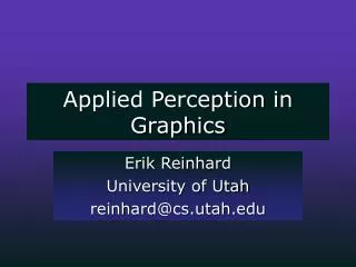
Applied Perception in Graphics Erik Reinhard University of Central Florida reinhard@cs.ucf.edu
Computer Graphics • Produce computer generated imagery that cannot be distinguished from real scenes • Do this in real-time
Trends in Computer Graphics • Greater realism • Scene complexity • Lighting simulations • Faster rendering • Faster hardware • Better algorithms • Together: still too slow and unrealistic
Algorithm design • Largely opportunistic • Computer graphics is a maturing field • Hence, a more directed approach is needed
Long Term Strategy • Understand the differences between natural and computer generated scenes • Understand the Human Visual System and how it perceives images • Apply this knowledge to motivate graphics algorithms
This Presentation (1) Reinhard et. al., “Color Transfer between Images”, IEEE CG&A, Sept. 2001.
This Presentation(2) Reinhard et. al., “Photographic Tone Reproduction for Digital Images, SIGGRAPH 2002.
Introduction The Human Visual System is evolved to look at natural images Natural Random
Color Processing Rod and Cone pigments
Color Processing Cone output is logarithmic Color opponent space
Image Statistics • Ruderman’s work on color statistics: • Principal Components Analysis (PCA) on colors of natural image ensembles • Axes have meaning: color opponents (luminance, red-green and yellow-blue)
Color Processing Summary • Human Visual System expects images with natural characteristics (not just color) • Color opponent space has decorrelated axes (but in practice close to independent) • Color space is logarithmic (compact and symmetric data representation) • Independent processing along each axis should be possible Application
Lab Color Space Convert RGB triplets to LMS cone space Take logarithm Rotate axes
Color Transfer • Make one image look like another • For both images: • Transfer to new color space • Compute mean and standard deviation along each color axis • Shift and scale the target image to have the same statistics as the source image
Why not use RGB space? Input images Output images RGB Lab
Color Processing Summary • Changing the statistics along each axis independently allows one image to resemble a second image • If the composition of the images is very unequal, an approach using small swatches may be used successfully
Global vs. Local • Global • Scale each pixel according to a fixed curve • Key issue: shape of curve • Local • Scale each pixel by a curve that is modulated by a local average • Key issue: size of local neighborhood
Global Operators Ward Tumblin Ferwerda
Global Operators Ward Tumblin Ferwerda
Local Operator Pattanaik
Spatial Processing • Circularly symmetric receptive fields • Centre-surround mechanisms • Laplacian of Gaussian • Difference of Gaussians • Blommaert • Scale space model
Scale Space (Histogram Equalized Images)
Tone Reproduction Idea • Modify existing global operator to be a local operator, e.g. Greg Ward’s • Use spatial processing to determine a local adaptation level for each pixel
Blommaert Brightness Model Gaussian filter Neural response Center/surround Brightness
Scale Selection Alternatives How large should a local neighborhood be? Mean value Thresholded
Tone-mapping Local adaptation Greg Ward’s tone-mapping with local adaptation
Results • Good results, but something odd about scale selection: • For most pixels, a large scale was selected • Implication: a simpler algorithm should be possible
Simplify Algorithm Greg Ward’s tone-mapping with local adaptation Simplify Fix overall lightness of image
Global Operator Results Our method Ward
Global Operator Results Our method Ward
Global Local Global operator Local operator
Local Operator Results Global Local
Local Operator Results Global Local Pattanaik
Summary • Knowledge of the Human Visual System can help solve engineering problems • Color and spatial processing investigated • Direct applications shown
Future Work This presentation
Acknowledgments • Thanks to my collaborators: Peter Shirley, Jim Ferwerda, Mike Stark, Mikhael Ashikhmin, Bruce Gooch, Tom Troscianko • This work sponsored by NSF grants 97-96136, 97-31859, 98-18344, 99-78099 and by the DOE AVTC/VIEWS